Accessing External Material Models for Magnetic Simulations

Characterizing magnetic behavior is crucial when designing magnetic devices involving ferromagnetic materials. Different materials (or the same material after certain processes) can react differently to the same stimulus and improper characterization can cause device failure. COMSOL Multiphysics® software version 5.2 expands the current support for describing magnetic materials and defines access to material models through external routines. Here, we demonstrate how this new functionality works in a case featuring hysteresis and review the current opportunities for modeling ferromagnetic materials.

Methods for Specifying Magnetic Models

In COMSOL Multiphysics, you can access a variety of constitutive relations for magnetic materials in all of the proposed formulations; i.e., Magnetic Fields, No Current; Magnetic Fields; Magnetic and Electric Fields; and Magnetic Field Formulation. These are sometimes called Vm, A, A-V, and T formulations, respectively.

When a new magnetic domain is added to an interface, the COMSOL® software assumes by default that this is uniquely characterized by a single quantity: relative permeability. This is adequate for most materials that are diamagnetic or paramagnetic because the relative permeability is very close to unity. Defining just the relative permeability may also be adequate for soft ferromagnets simply by entering a large number. If the permeability description is not rich enough, COMSOL Multiphysics offers specific features for defining it directly:

• The H-B curve or B-H curve in which data is stored in the material as look-up tables. The AC/DC Module includes 165 materials with such preloaded B-H/H-B curves.
• The Remanent flux density and Magnetization features, which are important for considering hard ferromagnets (i.e., permanent magnets) and hysteresis. In this blog post, we are going to focus on magnetization.

Like relative permeability, the other quantities can have arbitrary definitions and can be associated with the proper dynamical model. For example, magnetization can be associated with the solution of a PDE. This is shown in the Jiles-Atherton hysteresis implementation included in the Vector Hysteresis Modeling tutorial.

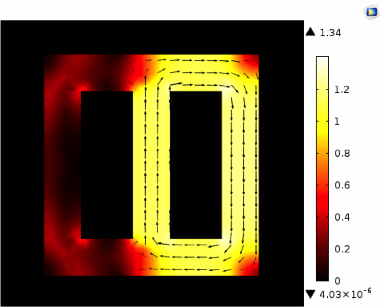
Simulation results for the magnetic flux density in the Vector Hysteresis Modeling tutorial.

What if your material model includes nonlinear expressions that are impossible or very difficult to express in terms of standard variables or additional partial differential equations (PDEs)? Version 5.2 of COMSOL Multiphysics features a new way to specify external material magnetic models. This feature supports any model that you would like to couple to the electromagnetic solution. Let’s learn more about this functionality…

The New External Material for Defining Material Models

Under the B-H curve and H-B curve nodes, you now have the option to connect the magnetic property of a specific domain to an external material. Among the external materials, there are two implementations that are specific to magnetism:

• General B(H) relation
• General H(B) relation

The first option is fitting for Magnetic Fields, No Current and Magnetic Field Formulation and the second option is suitable for Magnetic Fields and Magnetic and Electric Fields. Thus, COMSOL Multiphysics offers the same support for all magnetic interfaces.

There are a few reasons why you need these two distinct connected relationships. In Magnetic Fields, No Current and Magnetic Field Formulation, you compute from the dependent variable, the magnetic field H. The external material will output the value of the magnetic flux density, B, depending on the value from the magnetic field. In Magnetic Fields and Magnetic and Electric Fields, you compute from the dependent variable, the magnetic flux B. Thus, the constitutive relation has to output H as a function of B.

When you specify a formulation to compute the material data, COMSOL Multiphysics will call the native functions available in the shared library specified at the external material level. The library can be, for Windows® operating system, a dynamic link library (DLL).

You can run the models on Linux® operating systems and Mac OS X with proper compilation.

This action can be the result of compiling a C source code. The source code can contain extra state variables that you define in COMSOL Multiphysics. These state variables, including magnetization, enable communication between the material library and finite element model. Coded dynamics can be arbitrary, so at each iteration, magnetization and the self-consistent magnetic field and flux can evolve in such a way that follows a specific hysteresis model.

Another advantage to using source code is that you can distribute your models to colleagues and customers more safely and easily. With the Application Builder, you can even create easy-to-use apps that incorporate your external material functions and enable your colleagues and customers to see results. You can also preserve details of the material model for yourself, which is ideal for applications where certain details about the magnetic material may be restricted, such as micromagnetism, magnetic anticounterfeiting ink for banknotes, and military device demagnetization.

A naval military vessel is demagnetized by a deperming pier.

Material functions can also be written in other programming languages, making it easy for you to use legacy code instead of C code.

Putting New Functionality into Practice

To show you how the new magnetization functionality works, we have added a tutorial to our Application Gallery called External Material, AC/DC Module, General H-B/B-H Relation. The example includes a model file, a source C file, and a shared DLL that is compiled and linked for a 64-bit Windows® operating system. In this tutorial, we explain how to use the external material to reproduce what happens when you specify a B-H curve “from material” using the Soft Iron material in the AC/DC Module.

In order to explain the state variable, which can be defined in external materials, we will focus on a case that has the following hysteretic effects and features:

• An external material state variable, M, accounts for local magnetization.
• A Magnetic Fields, No Currents formulation. Thus, the external material computes the magnetic flux B as a function of the magnetic fields H and M. In this specific case, B = \mu_0(H + M).
• Dynamics for magnetization that would hardly be specified without a code.

First, we will deal with a scalar 1D case and then we will extend our example to a general vectorial 3D case. In 1D, we only need the x-component of the magnetization, magnetic field, and magnetic flux. These will be represented with M, Hx, and Bx, respectively. We will also need to find the magnetization and magnetic field at the last converged step, called with oldHx and oldM, respectively.

The dynamics for magnetization, M, include:

• Changing proportionally to the magnetic field with the proportionality constant, xi. M = oldM + xi * (Hx – oldHx).
• The magnetization modulus cannot increase above a certain value, Ms. If abs(M) > Ms, then M = Ms * sign(M).
• Decreasing only if the material is not saturated or if it is saturated and the local flux is opposite in sign to the local magnetization.

These dynamics would be pretty difficult to implement via a PDE interface, especially because of the conditional statements. But, as the figure below shows, this can be easily performed with a few simple instructions.

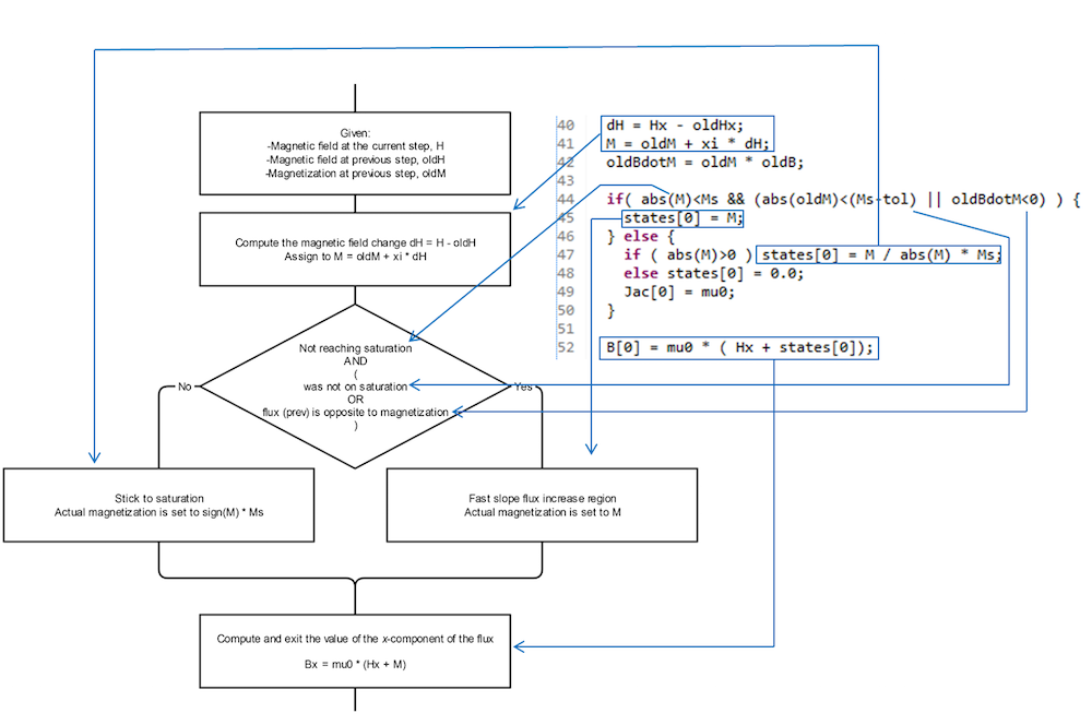
The flowchart and corresponding C code to implement the 1D scalar hysteresis model.

The model is nonlinear, as the resulting value of H may be too different from oldH so that a single iteration cannot find the proper solution that fits the Maxwell equations in all of the points of the space. The nonlinear convergence is automatically taken care of by the standard COMSOL Multiphysics solving engine. For very fast and robust convergence, we only need to specify \frac{\partial \text B_\text i }{\partial \text H_\text j}. This is a rank-2 tensor quantity whose components are stored in the variable “Jac” (Jacobian). For the present 3D model, it assumes a very simple expression, \text{ (1+xi)*}\mu_0\text * \delta_{ij} out of saturation and \text{ (1+xi)*}\mu_0\text * \delta_{ij}-\mu_0\text{*xi*}\frac{\text H_\text i\text H_\text j }{\text{(Ms)}^2} on saturation (\delta_{ij} is the Kronecker delta). In 1D, only the first component of Jac matters. Its value is \text{ (1+xi)*}\mu_0 out of saturation and \mu_0 on saturation. The Jac definition is included in both the scalar 1D and vectorial 3D codes.

Let’s see some of the results from this model. First, consider a 1D case where a sinusoidal uniform magnetic field is applied to a sample of such a magnetic material that is initially not magnetized. The magnetization would look like the results in the plot below.

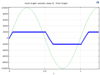
Results for a scalar 1D model. The green line signifies the externally applied magnetic field and the blue line with markers shows magnetization.

The corresponding magnetic flux would instead give the trajectory in the B-H plane shown below.

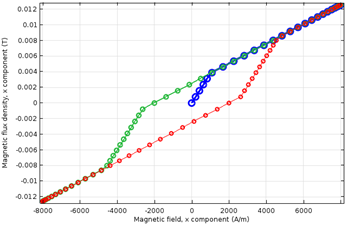
A scalar 1D model showing the dynamics of the magnetic flux, B, versus the externally applied magnetic field, H, during a sinusoidal cycle. The initial point is the origin and the dynamics follow in the order of blue, green, and red lines.

When the field is applied the first time, we follow the blue curve. Here, the flux increases rapidly up to reaching magnetization, Ms, and then it increases more slowly with the proportionality constant, \mu_0. This is the first magnetization curve.

When the magnetic field decreases from its maximum value to its minimum value, the magnetic flux follows the green curve downhill, which is the upper path of the hysteresis curve. The curve changes its steepness twice, once when the magnetic flux at the previous time step is negative, thus opposite in sign to magnetization (the magnetization value is Ms up until this point). During the fast slope region, the magnetization decreases. The second change in steepness is when the magnetization reaches –Ms. Then, magnetization freezes and a further decrease in the applied magnetic field causes the flux to change with the proportionality constant, \mu_0.

Finally, when the magnetic field increases to its maximum value, we follow the red curve, which is the lower path of the hysteresis curve. The paths of the green and red lines are similar. On the red line, the first change in steepness corresponds to when the magnetic flux becomes positive (as the magnetization is –Ms, thus negative, up until this point). After the second change in steepness, M = +Ms and the red curve brings the material to the same operating point where it was at the end of the first magnetization curve. Further cycles with identical amplitudes repeat indefinitely on the green line first and then the red line.

Despite being a simplified model that cannot account for some of the behavior of magnetic materials, it correctly features the expected hysteresis.

Notice that while moving on the green curve, if the magnetic field reincreases before the second change in steepness is reached, the magnetization starts to reincrease. Correspondingly, the flux follows the green curve up but does not experience hysteresis. If this behavior is undesired, changing the code can modify it.

We can now generalize the idea and the code to the case where the magnetization is a vector, which follows a new flowchart and code.

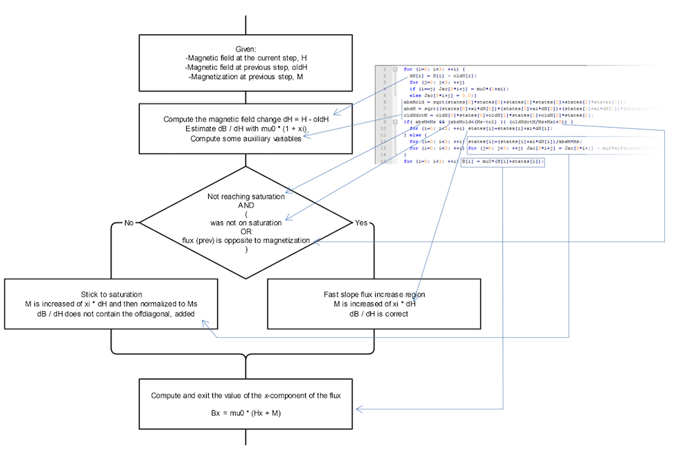
A flowchart and corresponding C code to implement the vectorial hysteresis model.

This code can be compiled just once, and it will work in 1D, 2D, and 3D. Let’s first look at how it behaves in a simple 2D case. Here, a square forces a magnetic flux in the horizontal direction. On the right of the square, there is a rectangular sample of the described hysteretic material. The plots below show the magnetization for two different scenarios.

The magnetic material is initially either not magnetized (left) or partially magnetized (right), with the external field first applied and then removed. Colored dots represent the magnetization with size (proportional to modulus) and color (representing the direction). The black and gray arrows superimposed on the colored dots represent the magnetization and magnetic flux, respectively.

In the scenarios above, the same color regions represent domains with a similar magnetization direction, highlighting the vector nature of the magnetization and magnetic domain formation. Despite the different initial configurations, the final configurations are similar.

In the plots below, the magnetization pattern is identical at the beginning, while it is very different after the pulse.

Now, the magnetic material is completely magnetized in the vertical direction and the external field is first applied and then removed. The case on the right has a stronger external field.

Next, we look at the B-H relationship for two points. In the plots below, the hysteretic B-H curves are clearly visible. They are much smoother than the previous 1D case, partly because the magnetization can rotate.

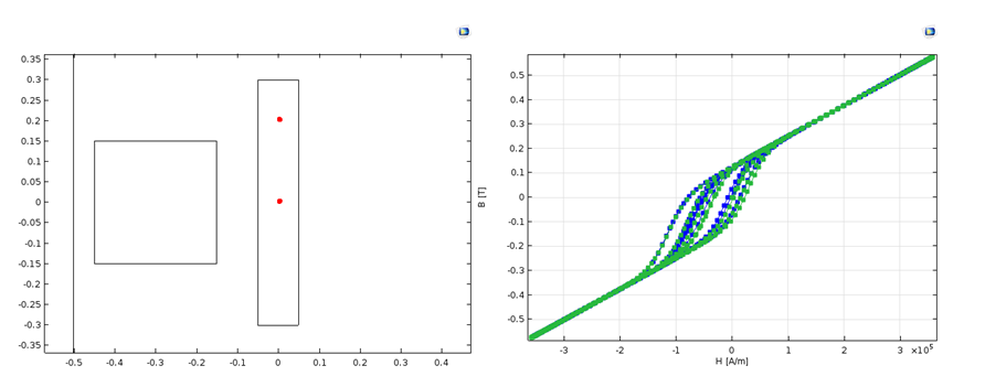
Left: The position of the two representative points. Right: A plot showing the B-H curve (x-components) for the lower point where the y-components are smaller (blue line) and B-H curve (y-component) for the higher point where the x-components are smaller (green line).

This same process works for more general cases. To demonstrate, let’s use the same external material in 3D. In the model below, a bobbin under a wrench creates a magnetic pulse.

Note that the material model is a General B(H) relation. To create the model, the geometry is split into two parts. In the lower part with the bobbin, we use a Magnetic Fields formulation. In the upper part with the wrench, we use a Magnetic Fields, No Currents formulation. At the interface, the fields are properly coupled.

A geometric configuration using the vectorial hysteresis model.

The wrench is made of the external magnetic material described here, and it is initially not magnetized. At the maximum current in the bobbin, the magnetic flux looks like that shown below.

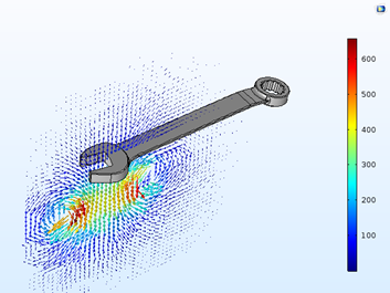
The magnetic flux at the maximum current in the bobbin. The vector lengths represent the magnetic flux in a log scale, while the color scale is linear.

After the pulse ends, some magnetic flux persists around the wrench due to the remanent magnetization, as shown in the figure and animation below.

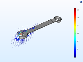
The magnetic flux when the current in the bobbin is finished. Vector lengths represent the magnetic flux in a log scale, while the color scale is linear.

The dynamics of the modulus of the magnetization during the current pulse in the bobbin.

Enhance Your Magnetic Simulations with External Materials

We have learned that with the new external material model, you now have extra options and freedom to define your magnetic materials. What we have shown here is a starting point for implementing different models, including empirical models such as Jiles-Atherton and Preisach, and models that are based on energy minimization, such as those used in micromagnetism.

Interested in exploring the use of external materials in your simulations?

• Download the tutorial: External Material, AC/DC Module, General H-B/B-H Relation
• Find more details on how to compile the C code for different operating systems in the section “Working with External Materials” in the COMSOL Multiphysics Reference Manual
• Contact us with any questions

Microsoft and Windows are either registered trademarks or trademarks of Microsoft Corporation in the United States and/or other countries.

Linux is a registered trademark of Linus Torvalds.

Mac OS is a trademark of Apple Inc., registered in the U.S. and other countries.