
Multiphase flow involves the simultaneous flow of fluids of different phases, such as gases and liquid, or solid particles suspended in a fluid. As such, modeling multiphase flow can require multiple approaches. One approach is to use a bubbly flow model to analyze the effects of bubble-induced turbulence. Here, we discuss a benchmark model of liquid and gas flow in a water-filled airlift loop reactor and validate the simulation results with experiments.
Improving Reactors and Multiphase Flow Techniques with Reliable Analysis
An airlift loop reactor is filled with water and injected with air bubbles at the bottom. Buoyancy causes the bubbles to rise, which creates circulation of the liquid. By modeling the induced turbulence in this type of bubbly flow model, you can predict the flow of liquids with dispersed bubbles, which is important in, for example, biochemical applications. Airlift loop reactors, such as airlift bioreactors, are useful for culturing microorganisms because they can create a relatively constant environment for cells and also provide a gentle form of stirring since cells are sensitive to mechanical stress.
Bioreactors that employ airlift bubble technology could potentially advance cell and tissue culturing techniques, such as culture aeration and disposable culture bags that simplify culturing and fermentation processes. In addition, scientists are developing new cancer treatments using bubble-based, jet-flow sorting techniques. T cells are cultured in bioreactors with hundreds of millions of cells and reintroduced into patients to identify and attack cancer cells. By using microvapor bubbles to generate air flow in the reactor, the sorting technique is gentle enough on the cells while retaining a speed of 5000 cells per second per single microfluidic channel.
In order to investigate the effects of bubble-induced turbulence in an airlift loop reactor design to advance reactor applications such as these, you can turn to simulation. The benchmark model discussed here is based on data from experiments published in peer reviewed scientific journals.
Modeling the Flow in an Airlift Loop Reactor
For the benchmark airlift loop reactor model, the liquid phase of the flow in the reactor is water and the gas phase is air. The model parameters are taken from experimental work and boundary conditions are set for the inlet, outlet, and symmetry:
- Inlet boundary condition: Two frits (glass components of the reactor design) at the bottom of the reactor, through which air bubbles are injected with a superficial speed of 0.015 m/s
- Outlet boundary condition: Free surface approximated by a slip condition for the liquid; the gas is able to exit the reactor through the outlet
- Symmetry boundary condition: Mirror symmetry invoked in the xy-plane at z = 0.04 m
Other boundaries are represented by the wall functions for the liquid and with zero gas flux for the bubbles. In addition to meshing the frits very finely, the mesh should be relatively fine in the interior of the reactor, since bubbles tend to create complicated flow structures.
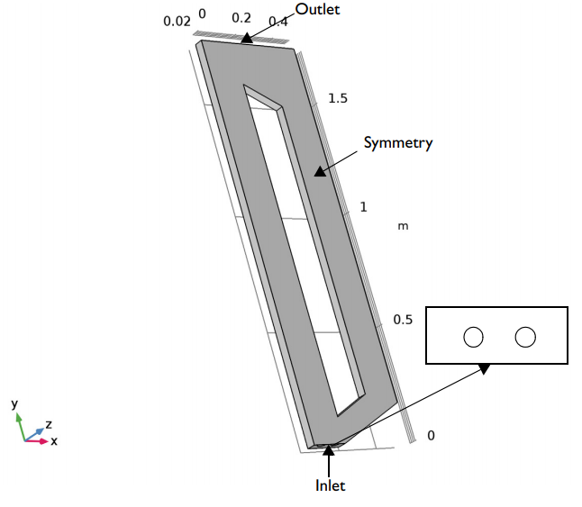
Model geometry for the airlift loop reactor.
Modeling the Flow
Next, the multiphase flow is set up using the Bubbly Flow interface available in the CFD Module, an add-on to the COMSOL Multiphysics® software. Instead of tracking individual bubbles, the Bubbly Flow interface tracks the averaged gas-phase concentration. This interface solves for the liquid velocity (the velocity of the continuous phase), pressure, and volume fraction of the gas phase and provides several slip models for the gas bubble (dispersed phase) velocity relative to the liquid phase. For this benchmark model, it’s best to use a pressure-drag balance slip model with a drag coefficient tuned for large bubbles.
When you model turbulence in bubbly flow, you need to account for the extra production and dissipation of turbulence due to the relative motion between the bubbles and the liquid by adding source terms to the turbulence equations. For example, if you take the equation for the single-phase turbulent model, k-ε, you can add a source term in the k equation, denoted by Sk. Other areas, such as turbulent transport, can be accounted for using the k-ε model.
One of the many advantages of the Bubbly Flow interface is its flexibility. You can turn the k-ε model on and off and control whether to include or exclude the bubble-induced turbulence term Sk. The interface for the physical model also has a default low gas concentration option, because, as indicated by reactor experiments, the gas concentration could be high.
Examining the Simulation Results
The results show the gas volume fraction and velocity streamlines for the liquid in the symmetry plane at t = 30 s. Other than a recirculation zone that is left out of the analysis, the results agree with the results of the reference experiment. As shown below, the maximum value of the gas concentration is about 7% closer to the two frits and higher than 2% in substantial parts of the reactor, which confirms that the low gas concentration assumption is not valid.
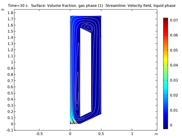
Gas concentration and liquid velocity in the reactor at 30 seconds.
Next, let’s examine the turbulent viscosity. After inducing turbulence with bubbles, there are relatively high levels of turbulent viscosity just above the frits. Levels are also high beneath the free surface, which could be why there’s no recirculation zone by the top-left corner. Another reason why the recirculation zone might be absent is because sloshing has been neglected in this example.
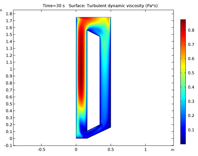
Turbulent viscosity in the symmetry plane.
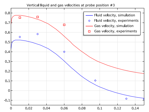
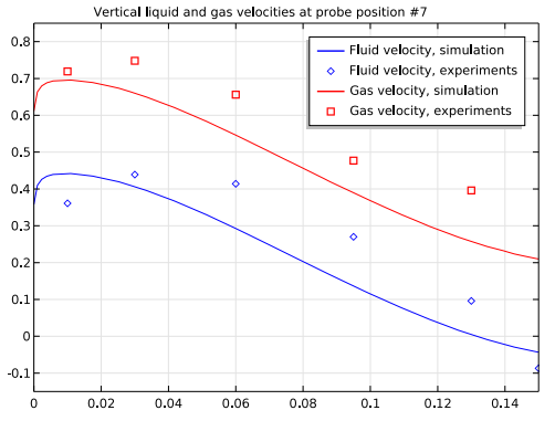
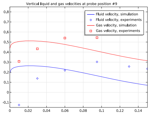
For the final result, we compare our simulation results with the experimental results for vertical velocities at the following probe positions: #3, #5, #7, and #9. Each probe position corresponds to lines in the symmetry plane at different, constant heights: y = 300 mm for position #3, y = 650 mm for #5, y = 1250 mm for #7, and y = 1650 for #9. The probes are positioned in the rising part of the reactor.
Looking at the plots below, we can see that at probe positions #3 and #5, which are in the lower part of the reactor, both liquid and gas velocities from the simulation are in close agreement with the experimental results. In the upper part of the reactor, the agreement at positions #7 and #9 isn’t as good — but this can be accounted for because, again, the recirculation zone at the top-left corner is left out of the simulation.
Comparison between the simulation results (blue) and experimental results (red) for vertical velocities at four different probe positions.
Keeping the many modeling assumptions used in this example in mind, we can consider the simulation results to be in good agreement overall with the experiment results, showing that CFD simulation is a valid method for airlift loop bioreactor design analysis.
Next Steps
Try this benchmark model yourself by clicking the button below. This button takes you to the Application Gallery, where you can download the MPH file.
Read More
- Check out this guide on choosing a multiphase flow interface
- Want more information on modeling reactors? Here are some topics to get you started:





Comments (0)