Application-Specific: Polar, Far-Field, and Particle Tracing Plots

In recent postprocessing blog posts, we’ve demonstrated different plot types that are typically used for common fluid, mechanical, chemical, and electrical applications. In the next several parts of this series, we’ll introduce a few more unusual plot types that are specific to unique applications and discuss some other tools that you can use to change the feel of your visualization. Here, we highlight polar, far-field, and particle tracing plots.

Polar Plots

Polar plots are exactly what you remember from math class. They use polar coordinates r and $\theta$ to describe a pattern, usually an acoustic or electromagnetic field. These plots are very useful for getting a localized or top-down view of the radiation pattern of your device. For instance, to ensure that a loudspeaker’s design is optimized for the most even sound distribution, you would examine a polar plot to see how the sound waves propagate from the speaker and what the range is.

To demonstrate this, I’ll show a polar plot from a conical antenna model. (If you have the RF Module installed, you can find this simulation under File > Model Libraries > RF Module > Antennas.) This model analyzes the impedance and radiation patterns of a conical antenna. The geometry of the antenna is shown below:

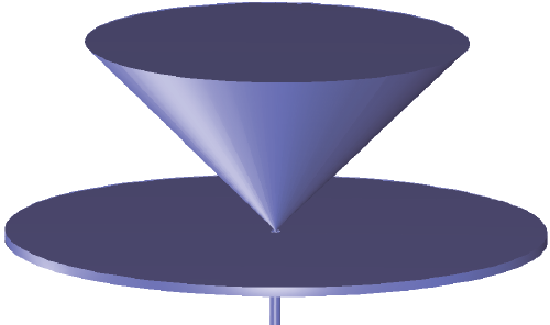
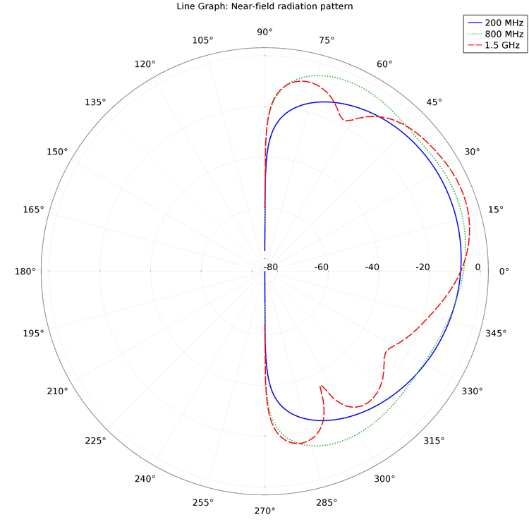
This antenna directs an electromagnetic wave propagating in a coaxial cable. Propagation occurs in the z-direction, and the model results show the radiation pattern close to the antenna for different frequencies. Below is a polar plot describing the near-field pattern changing with the elevation angle, $\theta$:

Far-Field Plots

In contrast to the plots just shown, a far-field plot describes a wave pattern (electromagnetic or acoustic) at distances far from the source. For instance, the far-field pattern of the conical antenna looks like this:

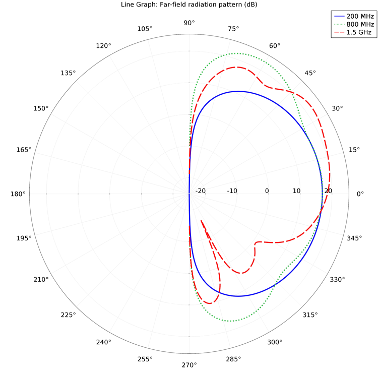
Comparing this to the near-field plot shown earlier, we can see how the radiation pattern changes with large jumps in distance from the antenna.

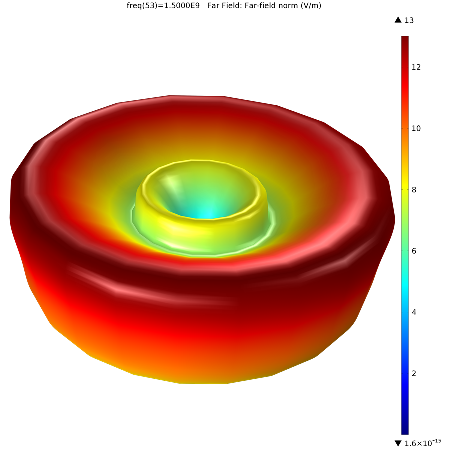
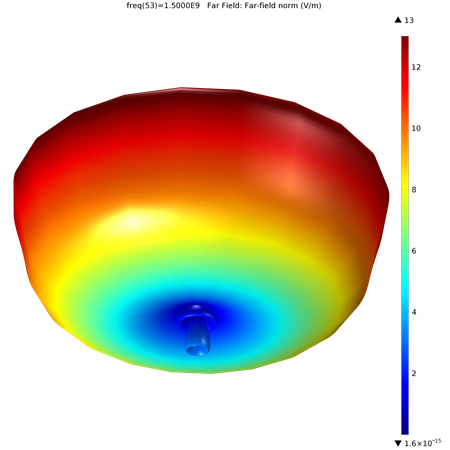
Far-field plots, however, are often shown in three dimensions, so these are not limited to the polar plot type. Variables are plotted for a chosen number of angles on a circle (in two dimensions) or a sphere (in three dimensions), where you can specify the angle interval as well as the origin and radius of the circle or sphere. This plots the radiation pattern by deforming the circle or sphere in the radial direction for each evaluation point specified. This means that the distance from the center becomes equal to the value of the expression on the evaluation point. (One advantage to this plot type is that the circle or sphere used for defining the plot directions is not part of the model geometry, so the number of plotting directions is unrelated to the solution domain.)

A 3D plot of the far field for the conical antenna is highlighted below. You’ll notice that this gives a very indicative view of the wave pattern, providing a sort of “big-picture” feel in contrast to the localized data in the polar plots.

Particle Tracing Plots

Lastly, there are a couple of plot types that are unique to particle tracing applications. These are the particle tracing plots, Poincaré maps, and phase portraits in COMSOL Multiphysics. To illustrate each of these plot types, I’ll use a model of a laminar mixer. If you have the Particle Tracing Module installed, this model can be found under File > Model Libraries > Particle Tracing > Fluid Flow.

The simulation analyzes fluid being pumped through a pipe with stationary blades. This type of mixing is suited for laminar flow because it generates only small pressure losses. The model evaluates the mixing performance by tracking the trajectories of particles suspended in the mixer.

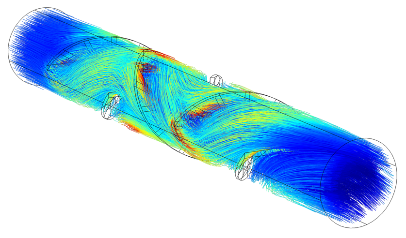
The particle tracing plot type shows the actual trajectories of a specified number of particles or a specified density and diameter. In this case, a species is dissolved in room temperature water. In the results shown below, a line tracks each particle five seconds after being released into the mixer. The color expression is based on the shear rate (1/s) of the flow.

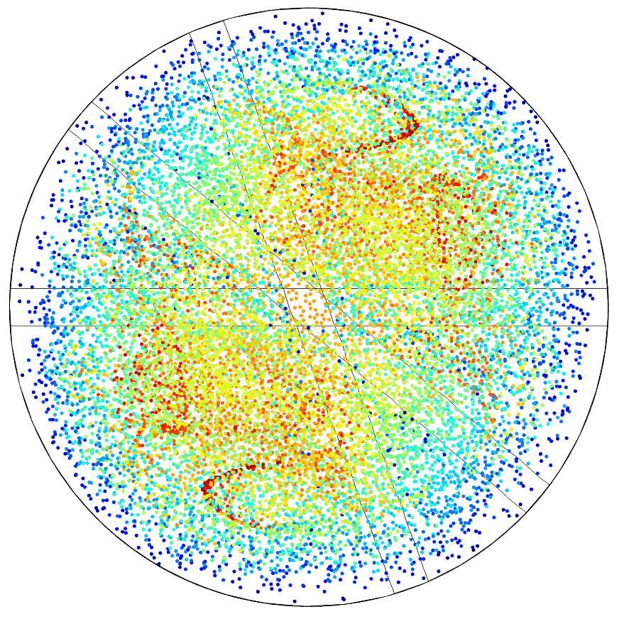
Another 3D plot group included in this model is a Poincaré map, or a first recurrence map. These are 2D plots that are created from a cut plane defined on the particle data set. This is used for visualizing the position of particles in a section transversal to their trajectories. The Poincaré map represents the particle trajectories in a space dimension that is one dimension lower than the original particle space. The plot shows a dot on the cut plane everywhere that a particle has crossed the plane (including multiple locations for the same particle if it crosses the plane multiple times). In the plot below, the dot color indicates the velocity of the particle when it crosses the plane, five seconds after release.

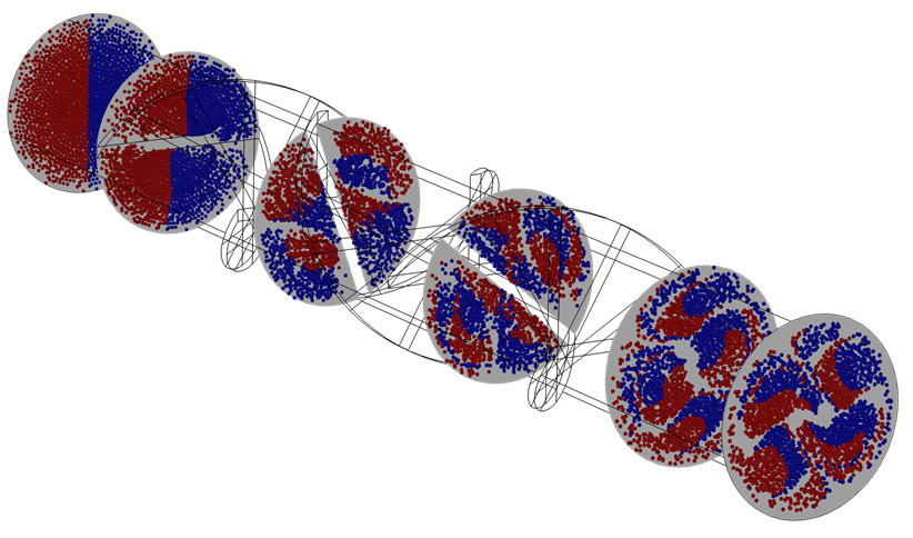
One nice trick to showing Poincaré maps is to include several of them in a 3D plot group. For instance, the results plot below depicts maps at different locations along the mixer, with the outlines of the blades underneath. In this case, the color of the dots indicates the level of dissolution (how well-mixed the species is in the water):

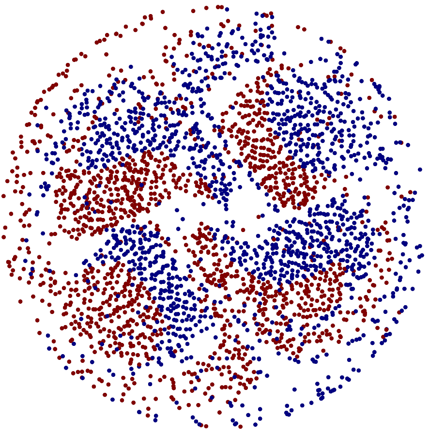
The very last plot type we’ll discuss here is a phase portrait. Like a Poincaré map, phase portraits show the locations of particles on a 2D plot. However, they are not necessarily on a plane with an orientation that is transversal to the direction of particle travel. Phase portraits are typically used to plot particle position and velocity together, where the position is taken as the distance from the origin. Below is a phase portrait depicting particle positions at t=5 seconds:

That’s all for the application-specific plot types. Hopefully you’ve enjoyed this introduction to some unique ways to show results and gather data in RF, acoustic, and particle tracing simulations. Stay tuned for our next blog post on creating deformations in your results plots!

Model Downloads

• Conical Antenna
• Particle Trajectories in a Laminar Static Mixer