
Today, we will introduce the concept of structural stiffness and find out how we can compute the stiffness of a linear elastic structure subjected only to mechanical loading. In particular, we will explore how it can be computed and interpreted in different modeling space dimensions (0D and 1D) and which factors affect the stiffness of a structure.
What Is Structural Stiffness?
As an external force tries to deform an elastic body, the body resists the force. This resistance is referred to as stiffness. We often casually use this term as a material property, whereas in reality, it could be a property of various geometric and material parameters. We will explore these cases here.
Before we dive in, we need to define stiffness mathematically. Let’s assume that a force, F0, acting on a body deforms it by an amount, u0. If we require a small force, ΔF, to deform the body by an infinitesimally small amount, Δu, then the ratio of these two quantities would give us the stiffness of the body at the operating point denoted by the state variables F0 and u0.
This is the definition of linearized stiffness, which can, in general, be used on both linear and nonlinear force versus displacement curves. The force-displacement relationship and linearized stiffness can be mathematically expressed using the following equations, respectively:
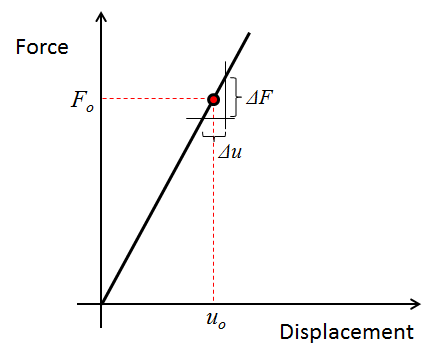
A typical force vs. displacement curve for a linear elastic structure.
An Example Problem
When modeling various types of structural systems, one of the goals of the analysis could be to come up with an effective value of stiffness and interpret its scope based on how we compute it from the structural problem at hand. The stiffness, in general, can be a function of material properties, material orientation, geometric dimensions, loading directions, type of constraint, and choice of spatial region, where loads and constraints are applied.
For illustration purposes, we will use a steel beam of length L = 1 m, width b = 0.2 m, and thickness t = 0.1 m. The face of the beam that is parallel to the yz-plane and located at x = 0 is rigidly fixed (i.e., zero displacements in x-, y-, and z-directions). The face that is parallel to the yz-plane and located at x = L has a uniformly distributed force acting on it. All other faces of the beam are unconstrained and unloaded. Consequently, they are free to deform.

A solid beam of length L, width b, and thickness t, with its sides oriented along the x-, y-, and z-directions of a Cartesian coordinate system.
We will compute the stiffness of this beam both analytically and using COMSOL Multiphysics, comparing the solutions obtained from these two methods.
Exploring Modeling Space Dimensions
When starting to model a structure, one of the critical choices that we need to make is deciding on how much detail we are really interested in. In other words, we need to determine if we can lump the entire structure as a single point in space or if we need to resolve it in one, two, or even three dimensions to get more details of spatial variation in certain quantities of interest. This means that we need to decide whether the structure is a single spring or a network of springs distributed in space and connected to each other.
To do so, we should try to answer the following questions — and possibly several others depending on what the modeling objective is:
- Is there any spatial inhomogeneity in the material properties?
- Is there any spatial inhomogeneity in the applied force?
- Do the geometric dimensions of the structure vary irregularly in certain directions?
- Are there any planes of symmetry that we can identify based on the symmetry in the modeling geometry, applied loads, and expected solution profile?
- Are there any localized effects, such as around holes or corners, that we are interested in?
- Can we neglect the stresses or strains in certain directions?
Stiffness in 0D Models
We will start by looking at a 0D model of the beam where all effects related to loading, deformation, and material response are lumped into a single point in space and the entire beam is modeled as a single spring.
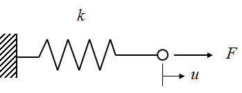
A 0D representation of the beam using a lumped stiffness, k, with a force, F, acting on it that produces a displacement, u. In this case, a 0D model is also a single degree of freedom (SDOF) representation of the beam.
Assuming that steel behaves as a Hookean solid (i.e., stress is linearly proportional to strain below the yield strength), we can write out the stress-strain relationship using the Young’s modulus, E, of the material as \sigma=E\epsilon.
Using a simplistic definition where stress is equal to force per unit cross-section area, \sigma=F/A, where A=bt, and strain is equal to the ratio of deformation to the original length, \epsilon=u/L, and combining these, we get F=(EA/L)u. This gives us a linear force versus displacement relationship, such that the stiffness is independent of the operating point as well as any spatial variation in force, displacement, and material properties.
Hence, we can express the axial stiffness of the beam for this 0D model with the following equation:
Assuming the Young’s modulus of steel is 200 GPa, we find that the axial stiffness of the beam is k = 4×10⁹ N/m.
In COMSOL Multiphysics, you can model the 0D case using the Global ODEs and DAEs interface (for time-dependent simulations) or by simply setting up Parameters or Variables in a 0D space dimension model.
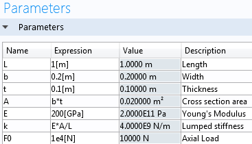
Screenshot of the Parameters table in the COMSOL software.
Stiffness in 1D Models
In reality, we know that the beam is fixed at one end, while the force is being applied at the other. Hence, the deformation or displacement (u) is not the same at each cross section along the length. In order to incorporate this effect, we would need to create at least a 1D model.
Computing Axial Stiffness
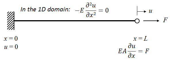
A 1D representation of the beam, obtained using the balance of static axial forces in the body.
A 1D model would require us to solve for the axial force balance equation on a 1D domain that represents the beam in order to find out the axial displacement (u) as a function of the x-coordinate that defines the 1D space. The axial force balance equation (ignoring any bending or torsional moment) can be written as:
with the boundary conditions at the two ends as u=0 at x=0 and E\frac{du}{dx}=\frac{F}{A} (Hooke’s law) at x=L.
Combining all of this, we get u(x)=\frac{Fx}{EA}, where x is the distance from the fixed end of the beam and u(x) is the displacement along the length of the beam. The 1D model represents an infinite number of springs connected to each other in series. This allows us to get more detailed information on spatial variation in displacement, stresses, and strains in the beam. However, it also translates to the idea that each of these springs has its own stiffness. Assuming that the Young’s modulus and cross-section area do not vary along the length of the beam, if we discretize the beam into n-number of springs in series, in our case, the stiffness of each spring (ki) will be k_i=nEA/L.
However, if we want to relate the 1D model with the 0D model, we have to imagine that the entire beam is being approximated by a single spring. Therefore, the equivalent stiffness in 1D would be the ratio of the maximum axial displacement and the axial force at the location where the force is being applied. In this case, u would be maximum at x = L where its value would be u_{max}=FL/EA. This gives us the equivalent single-spring stiffness of the 1D beam as:
This indicates that for the given modeling parameters, the solution (k = 4×10⁹ N/m) of the 1D model tends to be that of the 0D model when evaluated at x = L.
Computing Bending Stiffness
An additional advantage of moving over to a 1D model is that we can now explore the effect of loading direction. Although we restrict ourselves in a 1D space, we can compute the out-of-plane displacements v and w, respectively, along the “invisible” y– and z-directions when a force acts on the beam along these directions. Note that based on the chosen boundary conditions (clamped-free beam), the displacement components v and w would vary as a function of the x-coordinate.

A 1D representation of the beam, obtained using the balance of bending moment in the body.
Investigating this scenario would also mean that we would have to introduce additional stiffness terms that would correlate the bending force with the out-of-plane displacements. This would require us to solve the following moment-balance equation:
with the boundary conditions
at x=0; w=0 and \frac{dw}{dx}=0
and at x=L; \frac{d^2w}{dx^2}=0 and -EI\frac{d^3w}{dx^3}=F
In these equations, we have used the displacement (w) along the z-direction for representational purposes. The same idea holds true for the displacement (v) along the y-direction as well. Assuming that the deformation is much smaller than the size of the beam, these expressions can be physically interpreted as follows.
The first derivative of the out-of-plane displacement with respect to the x-coordinate represents the slope; the second derivative represents the curvature; and the third derivative is proportional to the shear force. In these equations, the term I denotes the second area moment of inertia and is a function of the direction about which the beam bends. For bending about the y-axis (i.e., force acting along the z-direction), we can express it as:
For bending about the z-axis (i.e., force acting along the y-direction), we can express it as:
Combining all of this, we get:
Therefore, the equivalent bending stiffness in 1D would be the ratio of the maximum out-of-plane displacement and the bending load at the location where the force is being applied. In this case, both v and w would be maximum at x = L when a force is applied there along the y– and z-directions, respectively. This gives us two possible equivalent single-spring bending stiffnesses of the 1D beam depending on the loading direction.
The force and displacement along the y-direction can be correlated using the stiffness k_{yy}=\frac{Eb^3t}{4L^3}. The force and displacement along the z-direction can be correlated using the stiffness k_{zz}=\frac{Ebt^3}{4L^3}. For the given modeling parameters, kyy = 4×10⁷ N/m and kzz = 1×10⁷ N/m.
Computing Stiffness in COMSOL Multiphysics
In COMSOL Multiphysics, you can set up the 1D model by first choosing a 2D or 3D space dimension and then using either the Truss or the Beam interface.
Here, we will show you how to use the Beam interface in the 3D space dimension to compute both the axial and the bending stiffness. The 1D structure will be modeled as an Euler-Bernoulli beam. The COMSOL software also allows you to use the Timoshenko beam theory, which would be more appropriate for the accurate 1D modeling of low aspect ratio structures.
Here is the workflow for obtaining the stiffness from the 1D model:
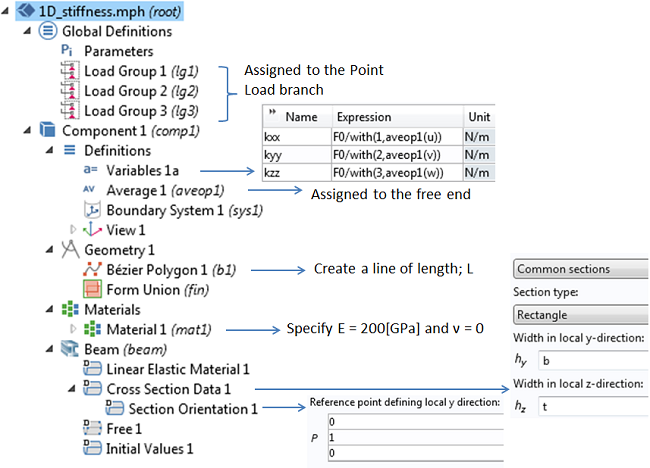
A snapshot of the 1D model made using the Beam interface. Variables are defined to evaluate the axial stiffness (kxx) and bending stiffness (kyy and kzz). An Average Coupling Operator is used to evaluate the displacements at the point x = L. The with() operator is used to fetch the solution from the different load cases that the model is solved for.
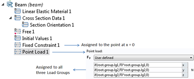
A snapshot of the boundary conditions used in the Beam interface. The Point Load branch is assigned to the point located at x = L.
In this model, we use a force (point load) of F0 = 1×10⁴ N. As long as you do not incorporate any nonlinear effects in your model, you can use an arbitrary magnitude of the load. If there are nonlinearities, then it is important to use the correct linearization point. Such cases will be discussed in a future blog post.
As shown here, you can create a “switch” using the if() operator and the names (such as root.group.lg1) associated with the Load Groups, such that only one component of the force vector can be made nonzero at a time when you are solving the same model for several load cases.
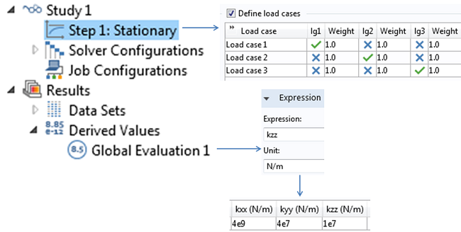
A snapshot of the Study settings illustrating how the load cases are set up to activate only one component of the force vector at a time. A Global Evaluation is used to print the values of kxx, kyy, and kzz. The COMSOL software solutions match the analytical solutions exactly.
The approach shown here for evaluating the stiffness components is applicable as long as we do not expect any coupling between extension and bending, (i.e., when the stiffness matrix is diagonal). We will present a more general computational approach in Part 2 of this blog series.
Next, we can solve the same model using the Timoshenko beam theory. As expected, this would yield the exact same result for the axial stiffness (kxx = 4×10⁹ N/m), but the transverse stiffness will be smaller than what we obtained from the Euler-Bernoulli theory. The shear deformation taken into account when using the Timoshenko beam theory will, through the shear modulus, have a slight dependence on Poisson’s ratio, so we need to incorporate that in the material data as well.
| Poisson’s ratio | kxx[N/m] | kyy[N/m] | kzz[N/m] |
|---|---|---|---|
| ν = 0 | 4×10⁹ | 3.91×10⁷ | 9.94×10⁶ |
| ν = 0.3 | 4×10⁹ | 3.88×10⁷ | 9.92×10⁶ |
Concluding Thoughts
Here, you have seen both analytical and COMSOL solutions to computing stiffness of linear elastic structures in 0D and 1D. Next up, we will talk about 2D and 3D cases.
Editor’s note: We published a follow-up blog post on this topic on 4/4/14. Read Part 2 to learn how to compute the stiffness of linear elastic structures in 2D and 3D.


Comments (6)
Badri Suhaini
February 5, 2016Hi, thank you for writing this blog. I have a question.
Is stiffness the same as elasticity matrix?
I have been trying to obtain the elasticity matrix of PMMA from the internet but I could not obtain it. I realized that the only way for me to obtain it is by calculating it using COMSOL. But I just want to know is this blog talking about elasticity matrix since it is stiffness?
Regards,
Badri
Daniel Burt
March 11, 2016Hi Badri,
The elasticity matrix as far as I know defines the effective Young’s Modulus in various directions for an an-isotropic crystal so essentially yes but only for anisotropic materials.
Ahmed Mohamed
February 1, 2017How can I put the real number of stiffness constant to a membrane?
Caty Fairclough
February 7, 2017Hi Ahmed,
Thank you for your comment and interest in this blog post! For questions related to your modeling, please contact our support team.
Online support center: https://www.comsol.com/support
Email: support@comsol.com
Best,
Caty
vikash kumar
February 10, 2017hi
i am doing uniaxial compression test simulation of polymer (ABS material ). i want stress v/s strain graph of the above . can anyone help me in finding out?
Samuele Martinelli
February 6, 2024For some reason my results are off scale… My global evaluation is (in N/m) kxx=4, kyy=0.04, kzz=0.01, same when computing with Timoshenko beam theory… It looks like I did everything correctly so I don’t understand why it is wrong. The numbers themselves seem correct, but they are totally off scale.
The things that are different are:
*In COMSOL 6.2 there is no bezier polygon, so I used a line segment
*The material section asks for density, but this does not seem to affect the model, I set it to 0
Everything else is the same…