When designing inductive devices, both challenges and possibilities are associated with the nonlinear behavior of ferromagnetic materials. COMSOL Multiphysics is well-adapted to the solution of highly nonlinear numerical models but high-fidelity modeling of nonlinear inductive devices also requires accurate material data. To meet this challenge, a library of 165 nonlinear magnetic materials is provided in COMSOL 4.4, bringing new powers to the design and modeling of electric motors, transformers, relays, etc. Here, we will discuss how the modeling process is facilitated by high-quality saturation curves that have been sampled and preprocessed especially for efficient and robust use in numerical simulations.
About Magnetic Saturation Curves
A common assumption in modeling is that a material responds linearly with respect to an applied stimulus as long as that stimulus is not too large. For example, Ohm’s law stipulates a linear relation between electric field strength and current density in a conducting medium;
a relation that, for many materials, is surprisingly accurate over a wide range of electric field strength.
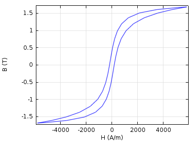
In this respect, ferromagnetic materials are fundamentally different as the level of magnetization depends nonlinearly on the magnetizing field, even for small values. There is also a dependency on the magnetization history (hysteresis) that is demanding and difficult to include in simulations. An example of a steady-state hysteresis loop is shown below.

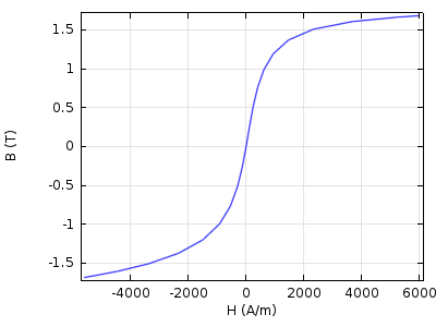
Trying to capture this in a material model for design and simulation is possible, but generally leads to very long simulation times. Another major challenge is that the parameters of a hysteresis model are not directly measurable but have to be found through elaborate curve fitting methods. For most design purposes, only the average B-H curve, which incorporates magnetic saturation effects, but not hysteresis, is needed:

Measuring B-H curves involves expensive equipment and requires considerable skill and experience, and published B-H curves are most often provided only graphically. When digitizing such curves, it is important to acquire enough data pairs and to avoid introducing too much digitizing noise.
Seen from the modeling and simulation perspective, for numerical efficiency and stability a B-H curve should be smooth, without local maxima or minima, and extrapolate correctly as in the saturation limit the slope of the B-H curve should approach the permeability of free space.
Thus, the new nonlinear magnetic materials database contains B-H curves that are densely and accurately sampled, have the hysteresis effects averaged out, and extrapolate correctly in the saturation limit.
Using a Nonlinear Magnetic Material in a Model
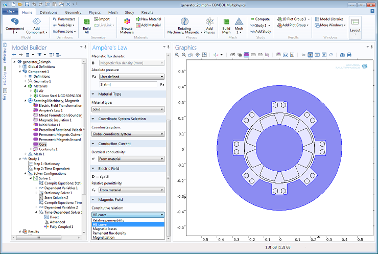
The nonlinear magnetic materials are available in a dedicated section in the “Add Material” dialog in the COMSOL user interface. Here we use it for the soft magnetic core in a model of a generator with permanent magnets in the rotor. Bringing up the Add Material window, there is a Nonlinear Magnetic section available.
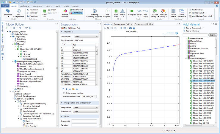
Once added to a model, the B-H curve is accessible for plotting (first quadrant):
and for use in the model:
Depending on the magnetic formulation used in the model, either the B-H curve or, as here, its inverse, the H-B curve is used. Both are provided by the nonlinear magnetic library materials together with electrical permittivity and conductivity.
Concluding Remarks
Altogether there are 165 materials falling into the following categories: Silicon Steels, Non-Grain Oriented; Silicon Steels, Grain Oriented; Metglas, Nano; Cobalt Steels; Nickel Steels; Stainless Steels; Low Carbon Steels; Castings; Powder Iron Core; Alloy Powder Core (including Ferrites). These are virtually available at your fingertips with the AC/DC Module and COMSOL Multiphysics version 4.4.


Comments (7)
Lingling Tang
December 3, 2013Dear Olsson,
I am now using COMSOL 4.3a, and always being restricted by the limited ferromagnetic material during modeling.
I wonder how can I get access to those 165 materials on my 4.3a software platform without update to 4.4 version?
Best regards!
Magnus Olsson
December 4, 2013 COMSOL EmployeeDear Lingling,
As for all other new functionality, the nonlinear magnetic library is only provided with the latest version. However, if you have installed version 4.4 but wish to use the BH-curve for a particular material in some other context, for example in an older version, you can always export the raw data to a text file and take it from there.
Best regards,
Magnus
AH
January 15, 2014Dear Magnus
Where can I find the .mph File for the shown simulation?
Thanks in advance
AH
January 15, 2014Dear Magnous
Do you have another model for Motor and not genrator ?
Sachin Umbarkar
August 12, 2016Dear Magnus Olsson,
Today’s talk was really informative and productive for our understanding. Also would like say …The concept of UWB antenna modeling using COMSOL multiphysics is quite lengthy and far field calculation for short duration electromagnetic applicatikn like Impulse radiating antenna design was depends on time domain calculation.
We request you to take more session on the above dedicated topic which will help us …
Also simplicity wise software needs more practical hand on training work
The software is really deep and interesting which covers large number of application with good accuracy.
Dr. Sachin B. Umbarkar
Premkumar Murugaiyan
January 10, 2017Dear Magnus Olsson,
The technical content is very good, especially the non-smoothened, non-linear B-H curves obtained from experimental techniques and need for fitting. I am a beginner in AC/DC module, can you please suggest some literature to carry out suitable curve fitting of my experimental saturation curve and including in COMSOL.
Magnus Olsson
February 2, 2017 COMSOL EmployeeDear Premkumar Murugaiyan,
There are many good text books on doing curve fitting using for example splines or using least squares methods to fit a parameterized function to a given data set. However, for this purpose (and in many other cases too), the challenge lies not so much in the fitting methods as those are pretty much standard. The challenge is rather to find a suitable function that is a good regularization. That is, it should be capable of providing a decent fit to your measured data but with the restrictions mentioned:
1) Not capable of exhibiting local maxima or minima.
2) Should extrapolate to a constant slope “mu0” in the high field limit.
There are magnetization models used for modeling hysteresis and/or magnetostriction that can be reduced to just describe magnetic saturation, e.g. using a Langevin function and fitting such a function to your data is one possibility.
That said, there is nothing magic added by curve fitting so unless you have to process a large number of measured BH-curves, making some manual adjustments to selected data pairs to remove local maxima/minima and adding a data pair at the end that makes the final slope right will in most cases be sufficient.
Best regards,
Magnus