Course: Modeling Electromagnetic Coils in COMSOL®

Looking for a quick, self-paced, guided introduction to electromagnetic coil modeling with the COMSOL Multiphysics® software and the AC/DC Module? We put together a course of video lectures that walk you through the modeling of electromagnetic coils, designed to show the key aspects of building such models. Let’s quickly review what’s in these videos and how to use the course to your best advantage!

Getting Started with Modeling Electromagnetic Coils

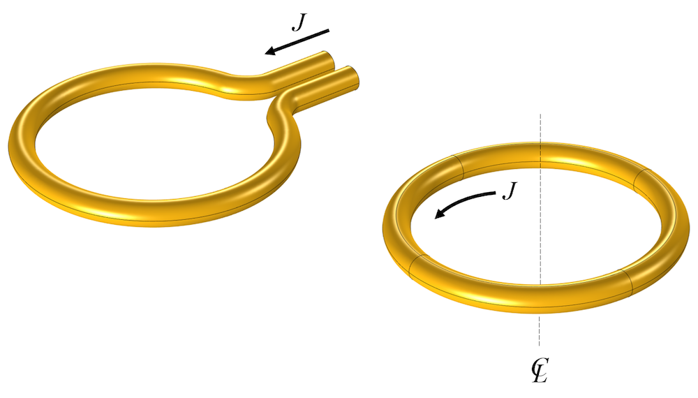
The simplest electromagnetic coil is a single turn of current-carrying wire, as you’ll see in almost any introduction to the topic. It’s often a reasonable engineering simplification to assume that the coil can be treated as a closed loop, meaning that it is axisymmetric, or invariant around the centerline.

A simple one-turn coil can also be modeled using a 2D axisymmetric assumption. 

It is with this assumption that our coil modeling course begins. For the first five parts, we will work in the 2D axisymmetric space.

Parts 1–5

In the first five parts of the course, we provide foundational knowledge regarding coil modeling and present information that is built on in the remaining sessions. We begin by building a model of a single-turn coil under DC conditions from start to finish. The air domain is bounded by an infinite element region. We consider 1 amp of current to be passing through the coil and model it in the 2D axisymmetric plane. We also provide some additional background as to why and how we can use the 2D axisymmetric assumption.

Upon computing the model, we also evaluate the coil conductance and coil resistance. We then progress to moving the coil into the frequency domain. We model the coil being excited with 1 Amp of current and assume that the excitation current variation is sinusoidal and occurring at a known frequency.

After building and reviewing the coil model in the DC and AC case, we discuss the potential modeling issues you should be aware of when building these types of models.

Thereafter, we continue to expand the coil model by simulating it being connected to an electric circuit. We do this by introducing a magnetic core as well as a secondary pickup coil through which some of the current flowing through the primary first coil is picked up from. We then show how to perform some postprocessing to visualize the current magnitude and direction between the coils.

From here, we venture into modeling coils containing multiple turns and different winding patterns. Additionally, we go over modeling coils up to and around the first resonant frequency as well as flat coils. We then end with a comprehensive overview of the Magnetic Fields physics interface and the different features contained therein that you can utilize when building coil models.

Once completing the videos in this introductory part of the course, you will have seen the foundations for 2D axisymmetric coil modeling techniques.

Electromagnetic Heating in Coils

One of the common uses of COMSOL Multiphysics with the AC/DC Module and Heat Transfer Module is for modeling inductive heating, the process by which a coil is used to heat up a workpiece over time. In the next five parts of the course, we address this topic in depth.

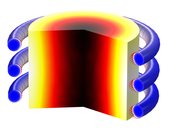
Workpiece being inductively heated over time, with nonlinear material properties. 

Parts 6–10

In parts 6 through 10 of the course, we demonstrate a full walkthrough of both setting up and solving inductive heating coil modeling problems. We begin by setting up a 2D axisymmetric model of a three-turn coil in free space and specify 1 kiloampere of current flowing through each turn of the coil. We also include a workpiece in the center made of a titanium alloy. The problem is modeled in the frequency domain at a constant frequency of 10 kilohertz. Upon computing the simulation, we perform some postprocessing to look at the losses in the workpiece part.

It is from here that we expand our initial electromagnetics problem into an electromagnetic heating problem. In order to find how the electromagnetic losses cause the temperature to rise and to what extent, we add a second physics, heat transfer, to the coil model. After, we show you how you can modify the material properties from using scalar, constant values to being a function of a model input (in this case, temperature). We then continue to expand the model by showing how to alter the heating profile of the workpiece over time as well as solve with multiple frequencies.

From there, we dive deeper into discussions on various topics regarding the solvers. We also address thermal modeling considerations not covered previously by including convection and radiation in the thermal model. We also demonstrate how to model the heating of moving parts.

Once completing this section of the course, you should be confident in addressing most coil heating problems.

Modeling of Forces, Motion, Nonlinearities, and More

The next five parts of the course address another kind of multiphysics: the coupling of electromagnetic forces to the deformation and motion of parts, such as in solenoids.

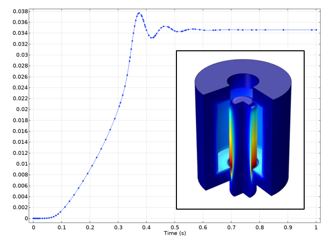
Displacement of a solenoid actuator over time. 

Parts 11–15

In parts 11 through 15 of the course, we build and work with several different coil model geometries to conduct various analyses. This is a departure from the previous parts, where we usually worked with a single geometry and model setup, but made changes to it to progressively make our models more complex and expand the analysis.

We begin by demonstrating how to model electromagnetic forces and do so accurately, which is accomplished through the addition of Force Calculation features to our model and then using Global Evaluation features to find the total force observed on the coils in the model. We then explore how to determine the accuracy of the force quantities that were evaluated, which is done quickly and easily through performing a mesh adaption. Through generating a plot afterward that displays the values of the force quantities as function of the mesh refinement, we observe if the force quantities start to converge to some value.

We move on to how to model a magnet moving and inducing currents within a coil. The magnet is defined using an Ampere’s Law domain feature, while the movement is defined using several of the Moving Mesh features in the software. In solving this model, we encounter some issues related to the solver settings, as a result of an inconsistency among the source term and initial values of the model, which we show how to address in detail.

From there, we move into modeling a reversed version of the previous problem, a solenoid actuator. This time, we have a coil and apply a time-varying current to it in order to induce movement in a part nearby. Thereafter, we demonstrate how to model an inductor with a nonlinear core material. While doing so, we touch on topics discussed earlier with previous models, such as solution accuracy and convergence. We also show you how to visualize the cycle-averaged loss in the core region by integrating our equation for the coil current, introducing another equation into our model through the Global Evaluation interface, and performing a global evaluation with use of the at operator.

Our session concludes with another model, where we take a coil and optimize that coil so that the B-field is uniform at the centerline of the geometry as much as possible. We demonstrate defining an objective function and improving the function by changing the current through the turns of the coil and the position of the coil.

Once completing this section of the course, you should be knowledgeable in modeling, computing, and evaluating forces, motions, and nonlinearities for most coil models.

Modeling of 3D Coils

The last five parts in the coil modeling course address issues related to modeling 3D coils. Although most of the concepts of coil modeling can be learned solely on a 2D axisymmetric model, there are some unique issues that need to be addressed in 3D.

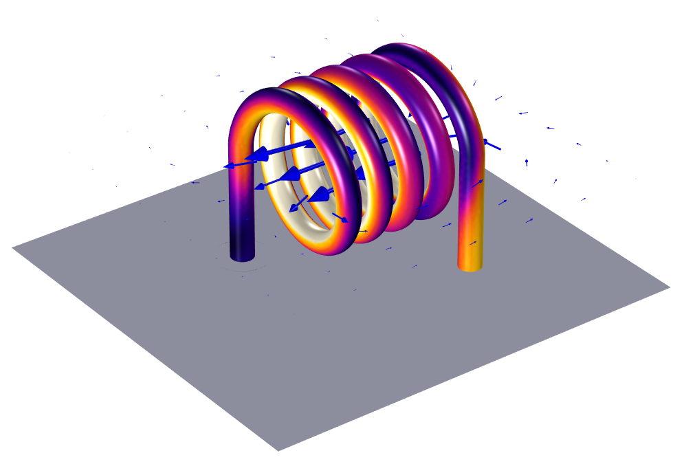
A 3D coil model showing current magnitude on the coil and the surrounding magnetic field. 

Parts 16–20

In parts 16 through 20 of the course, we set up our first 3D coil model, which we will solve in the stationary, DC regime. When building the geometry of our coil in 3D, we use a helix pattern and at the ends of the coil bends, extrude the coil into vertical straight tubes. In doing so, we show you some different approaches that you can use to ensure the coil geometry is a single domain. This can be done using the Delete Entities, Union, or Form Composite Domains operation, however, it is not required and is ultimately a matter of preference and bookkeeping. Adding a Coil domain feature to our model, unlike previously for our 2D axisymmetric coil models, includes a Geometry Analysis subfeature in which we need to specify where we want the current to flow both into and out of the coil.

Upon computing the model, we receive an error message, and then explain why and how this occurs and how to address it. A new study step, Coil Geometry Analysis, is included in our study to first compute the current direction through the structure. After successfully solving the model using the Magnetic Fields interface, we then solve the same problem using the Magnetic and Electric Fields interface.

After completing these models of a single conductor coil, we then go into demonstrating specialized functionality for modeling different types of coils. We discuss and show how instead of explicitly modeling the turns for multiturn coil, we can model a homogenized multiturn coil by using an approximately equivalent geometry and adjust the Coil domain feature settings. Other types of coils include thin, ribbon-like coils; tightly packed coils with no gap between the turns; and using an edge, wire coil geometry. The Part Libraries in the software contain several different types of built-in coils available for you to add and use.

We also introduce an infinite element region to the air domain of our coil model and go into detail discussing the use of this feature and what it physically represents. From there, we move away from the static, DC regime and move our 3D coil modeling into the frequency domain. We also go into coil modeling in the low-frequency, mid-frequency, and high-frequency regimes. Thereafter, we discuss how to handle some issues you may encounter with meshing and convergence for these models. Lastly, we demonstrate how to model resonance and handle couplings between coils.

Once you’ve gone through this last section of the course, you’ll have the foundations to solve 3D coil models. We hope that this material will educate and inspire you to build coil models in COMSOL Multiphysics and the AC/DC Module, and to do so faster and with confidence in your modeling!