
One of the issues in the computational modeling of fluids is the question of experimental correlation. Although it is very easy to generate beautiful 3D visualizations of the numerical results, comparing these to experimental results is often more challenging. One experimental technique is Schlieren imaging, which generates a set of 2D pictures of 3D flow fields. It turns out to actually be very easy to create a visualization of this type of imaging in the COMSOL Multiphysics® software. Let’s learn more.
Background on Schlieren Imaging
The story of the Schlieren imaging technique dates back ages; it might even predate written history. Ancient travelers over deserts and seas were familiar with the concept of a mirage, such as the fata morgana and far-away apparitions of objects like upside-down sailing vessels (which might have led to fables such as the Flying Dutchman). These phenomena occur because light rays bend slightly as they go through air of different density. This was probably understood in some form or another well over a millennium ago, but it is only in the last 500 years or so that experimental techniques were developed.
Although there are many variations to the Schlieren imaging method, the basic operating principle is quite simple. Any temperature or pressure variation within a fluid (or solid) will lead to a local variation in the density, and the density affects the refractive index. For atmospheric air, the Gladstone–Dale relation for the refractive index, n, in terms of the density, \rho , is:
Where, for visible light, G is about 0.23 cm3/g.
It should be remarked that the above expression is a simple starting point, but more complete expressions are available, and for gas mixtures and reacting flows, even more complicated expressions exist. The objective of the experimental method is to develop an optical image of these density variations within the flow.
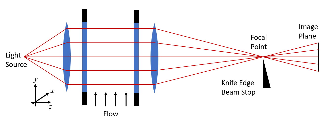
A Schlieren imaging setup.
A typical experimental setup is shown in the schematic above. Two transparent windows, such as on the sides of a wind tunnel, enclose a flow field. We begin by assuming no variation in the flow. There is a light source on one side, as well as some optical elements (lenses or mirrors) that give a uniform illumination. Using the geometric optics approach, we treat this light as a set of parallel rays that pass through the flow, and then through another set of optical elements that focus the light onto an image plane.
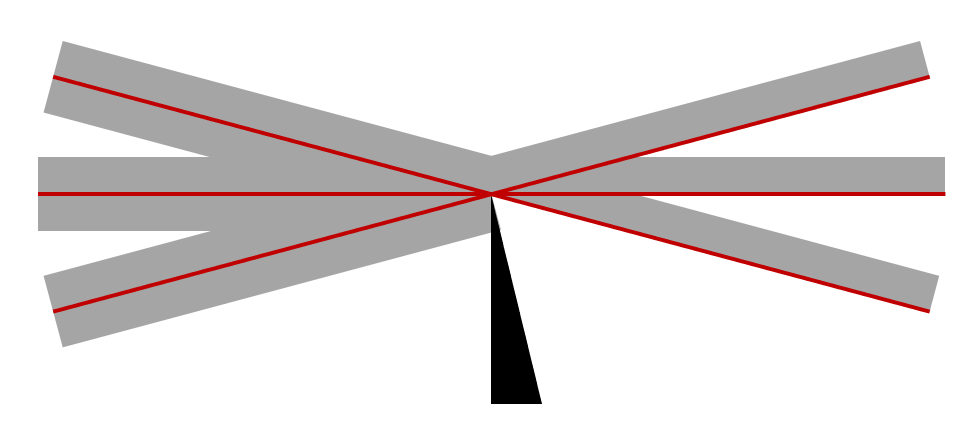
Unperturbed rays at the focal point. The knife edge blocks half the light, and diffraction at the edge is ignored.
It is important to realize, however, that the so-called focal point is not a single point. Light cannot be focused to a point; there will always be some finite radius to a focused beam. Understanding this point requires an understanding of wave electromagnetics.
However, for our purposes, it is sufficient to stay within a geometric optics approach as long as we understand one key point: An obstruction placed at the focal point occludes a fraction of the light. If we place a knife edge (experimentally, often a razor blade) at this point, then we can block half of the total light but still get the complete image, albeit at half the intensity. One way of thinking about this, which is convenient solely for the purposes of our understanding, is to consider each ray as having some finite thickness, as in the image above.
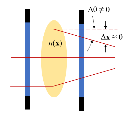
A region of slight variation in the refractive index will slightly alter the direction of the rays, but not their position at the exit plane.
Now, let’s consider what happens when there is a density variation in the flow. We know already that the refractive index is a function of density, so let’s introduce a small refractive index variation into our schematic and see what happens. The image above presents the key behavior. We will skip over the entire derivation and emphasize these points:
- A variation in the refractive index in the xy-plane will cause the beam to very slightly change direction (angle) as it propagates along the z direction
- We assume that the rays of light experience only a very negligible change in position in the xy-plane as they pass through the experimental domain
That is, any ray of light entering the domain at position (x,y) will leave the domain at the same position in the xy-plane but will be going in a slightly different direction. Let’s think about the consequences this has at the focal point. As we see in the image below, the variation in the refractive index slightly perturbs the rays, thus slightly more (or slightly less) light will be occluded by the knife edge. This shows up as light and dark regions on the image plane and forms the basic operating principle.
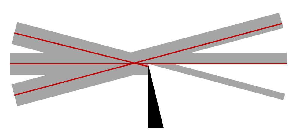
Perturbed rays at the focal point. The knife edge blocks differing amounts of light for rays incident at slightly different angles.
The knife edge can be rotated to be parallel to the x– or y-axis, or can be replaced with a pinhole beam stop, each resulting in different patterns of light and dark. These light and dark bands in the Schlieren image correlate to the following integrals through the flow domain:
| Obstruction Type | Equation |
|---|---|
| Knife edge parallel to x-axis | \int \frac{\partial n}{\partial y} \partial z |
| Knife edge parallel to y-axis | \int \frac{\partial n}{\partial x} \partial z |
| Pinhole occlusion | \int \sqrt{\frac{\partial n}{\partial x}^2 +\frac{\partial n}{\partial y}^2} \partial z |
As it turns out, these integrals are trivial to implement within COMSOL Multiphysics.
Implementation within the COMSOL® Software
Before we create our images, we need to touch on one of the aspects of computational fluid dynamics: the treatment of a compressible fluid. In short, for numerical modeling reasons, we often assume that the fluid has constant density. This is perfectly reasonable from the point of view of the flow model. A density variation of less than ~1% is likely not going to alter the solutions for the velocity or pressure fields very much, but it will quite measurably alter the refractive index. So, if you are modeling the flow assuming constant density, such as via the Boussinesq approximation, make sure to use the pressure field — and the temperature field if one is computed — to postevaluate the spatial density variation. For atmospheric air, the ideal gas law is appropriate to use, but make sure to do so in terms of absolute pressure, and not gauge pressure.
Once you have developed the expression for density variation within the modeling space, use that to compute the refractive index distribution as well as the derivatives of the refractive index in one or two directions. For this, the built-in differentiation operator is used. For example, if our expression for density is the variable rho, we can take the x-derivative as d(rho,x). We now only need to take the integral of this expression along the direction across the flow, and plot them onto a plane parallel to the flow. For this, we use the General Projection operator. We can even project onto a boundary outside of the flow domain, which can be quite advantageous if we want this operator to be evaluated using a finer mesh than the mesh that exists on the boundary of the flow domain.
We also need to consider what happens when there is an opaque obstruction in the flow. In these cases, we don’t want to evaluate the above integrals everywhere. We can use the Workplane Projection functionality, available in any one of the CAD Import Module, Design Module, or LiveLink™ products as of COMSOL Multiphysics version 6.0, to project the outline of any obstructions onto the optical exit plane boundary and only evaluate the integrals over the nonshadowed surfaces.
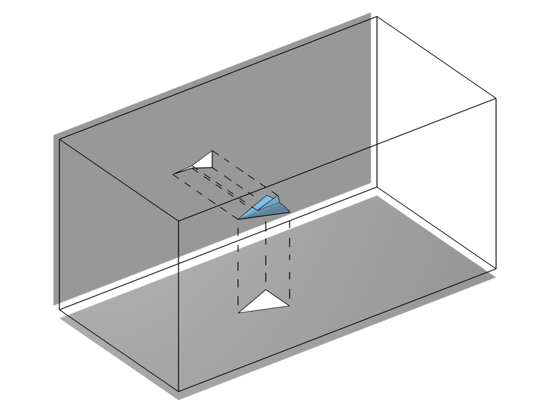
The Workplane Projection functionality, which projects the outline of a geometry onto a plane.
With these techniques in our modeling arsenal, we can make plots that correlate with the experimental results of a Schlieren imaging setup. The image below is of a high Mach number flow around an object, similar to that demonstrated in the Euler Bump tutorial model. This same technique can also be used for visualizing the results of acoustics models.
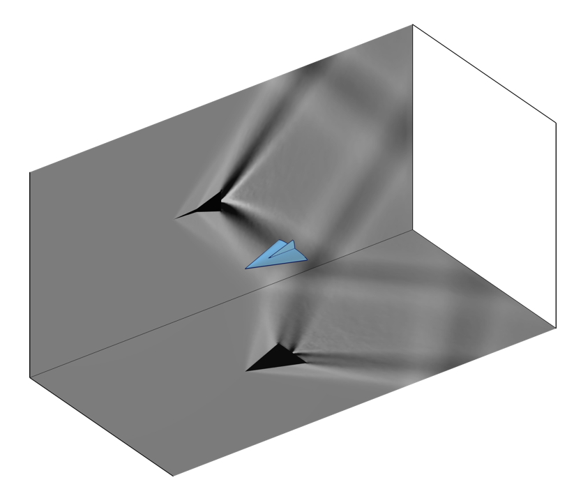
Images created via the General Projection operator that correlate to Schlieren imaging of a model in a transonic wind tunnel.
Next Step
Want to learn more about the software’s CFD modeling capabilities? Contact us!


Comments (0)