Equation-Based Modeling with a Space-Time Discretization

One of the core strengths of the COMSOL Multiphysics® software is that you can modify almost any expression in your computational model. This functionality must be used with care, but you can do great things with it. Let’s take a two-dimensional (2D) thermal model with translation, set some material properties to zero, and observe that this is analogous to solving a 1D transient model. We will then see how this makes some types of optimization problems easy and fast to implement.

Going from 2 Spatial Dimensions to 1 Spatial Dimension and 1 Time Dimension

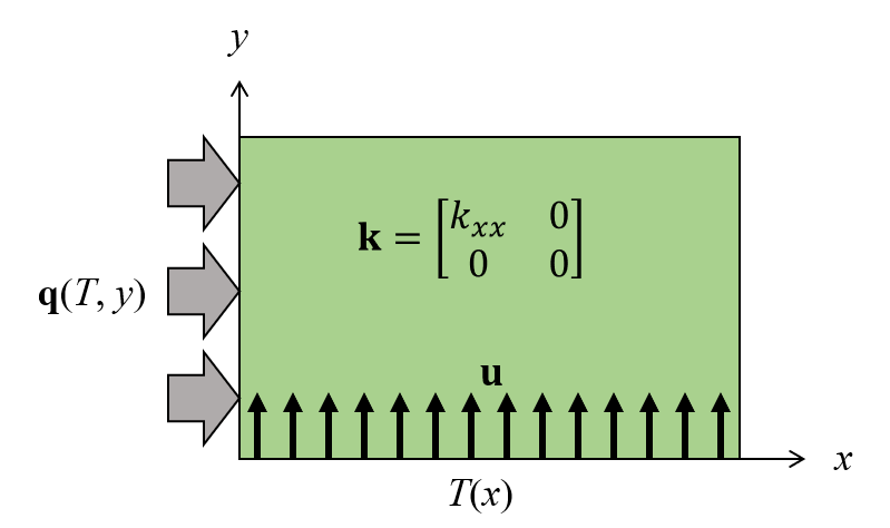
Schematic of a 2D stationary thermal model that is analogous to a 1D transient model.

Let’s consider a very simple-looking 2D heat transfer model of a rectangle. We will solve the stationary (time-invariant) heat transfer governing equation for temperature, T, in the absence of volumetric heating but with a convective term, \mathbf{u}, as follows:

Where \rho is the material density; C_p the specific heat; and \mathbf{k} is the thermal conductivity, which in this case is a diagonal matrix of the form:

It is helpful to write out the governing equation in a little bit more detail by expanding out all terms:

Now we will do something interesting: We will assume that the velocity vector is purely in the +y direction, so u_x = 0, and we will set the y-component of the diagonal thermal conductivity tensor to zero, k_{yy} = 0. Now the above equation reduces to:

Setting a term in the thermal conductivity tensor to zero might seem quite unusual, but it gives us an interesting benefit, which becomes apparent when we write out the 1D, transient, heat transfer governing equation without volumetric heating or a convective term:

Note that the first terms in the two equations above look almost identical, and if we choose the velocity term correctly, the two equations will be identical. So now we have something quite interesting: Our 2D stationary model appears to be the same as a 1D transient model.

In fact, the equations are identical, but when we solve them numerically, there are some things to be aware of. First, applying a fixed temperature condition at the bottom boundary of the 2D domain is analogous to the initial condition for the transient 1D case. Second, for such a 2D model it makes sense to have a mapped mesh (aligned with the y-axis) and the number of elements in the y direction can be thought of as a fixed time step. This is quite different from the time-domain model, which uses adaptive time stepping by default. The 2D model will also (by default) include numerical stabilization terms that will make the results slightly different between the two, unless one of the models went to a high level of mesh and tolerance refinement.

The next question is, of course: What can we do with this? To see how this can be useful, let’s look at a classic 1D heat transfer model where a slab of material is heated, as shown in the image below. Despite its apparent simplicity, a great many problems of engineering interest reduce to this classic case. As we heat the material from the left surface, the entire volume of material gets gradually, but nonuniformly, hotter. There is also radiative cooling and some free convection from the left side, approximated as a constant heat transfer coefficient.

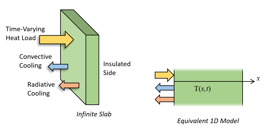
The transient heating of a slab of material can be reduced to a 1D model.

This problem can be solved in COMSOL Multiphysics by setting up a 2D rectangular domain and using the Heat Transfer in Solids and Fluids physics interface. Within this interface, you can apply a Translational Motion subfeature to the Solid feature, a Temperature boundary condition at the bottom boundary, Heat Flux and Surface-to-Ambient Radiation features along the left side to model convective and radiative cooling, and another Heat Flux condition to impose a heat load. Sample results with a uniform heat load over the time axis are shown below.

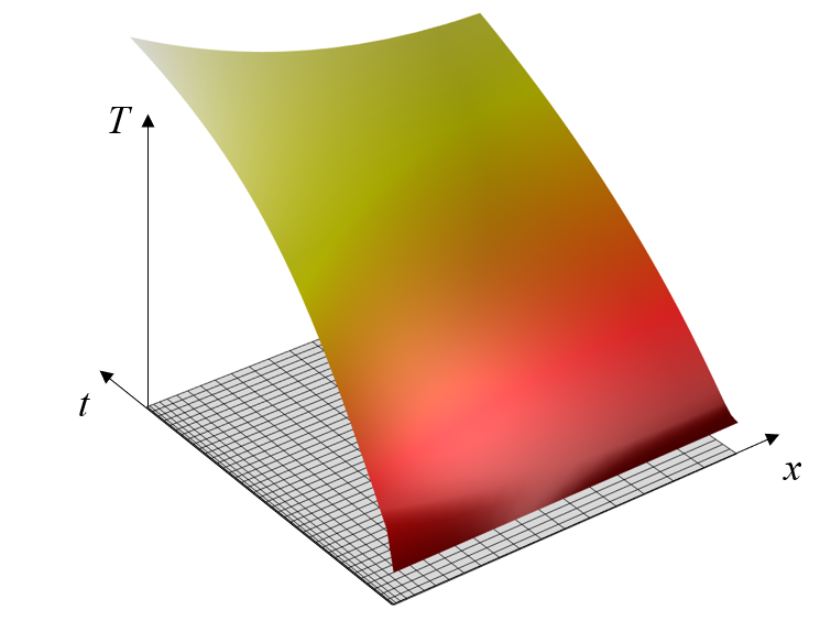
Sample results of a 2D stationary model representing the transient heating of a 1D slab. The mesh is shown as well.

Suppose now that we want to optimize this heating process. Let’s try to vary the imposed heat load over time with the objective that the temperature throughout the entire slab be as close to a target temperature as possible at the end of our simulation time, and also consider a constraint that the peak temperature never gets over a specified limit. By having a 2D version of our 1D slab, it turns out that this optimization problem is quite easy to set up. Let’s find out how!

Defining the Optimization Problem

The Density Model feature within the Topology Optimization branch of the Definitions is used to define the variable controlling the heat flux over time. This feature defines a field over a boundary that is constrained to be between 0 and 1, representing no heating and maximum heating. The discretization of this field is linear, meaning that over each element along the time axis the heat load can vary linearly, and thus the heat load could vary over a timespan determined by our mesh size in the y direction. This is not ideal — It implies the heat load is changing as quickly as our time step. We instead want the heat load to vary in time slower than our discretization. So we need to take one more step, and that is to introduce a Helmholtz filter. This is a popular idea in the field of topology optimization, and it available within the Filtering section of the settings. The Filter radius need simply be larger than the mesh size, and represents a smoothing time. The name of this filtered control variable field is dtopo1.theta, and multiplies the incident heat flux.

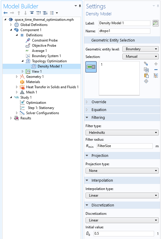
Screenshot of the Topology Optimization Density Model feature, defined along the heated side of the slab, and over the entire axis representing time.

Our objective expression is shown in the screenshot below, it is an Integral Probe over the top boundary (representing the final time.) The expression that is integrated is based upon the computed solution, T, and T_target, the temperature we want to get to. By defining an objective that is the integral of the squared difference between the computed and target temperature over this boundary, we have a differentiable function that has a minimum when the final temperature is as close as possible to the target. The name of our objective is comp1.obj, which we will refer to from the Optimization study step.

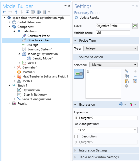
Screenshot of the Objective Probe feature, defined over the top boundary, defining the expression that is our objective to minimize.

We have a constraint, defined within the Optimization interface, that is:

comp1.constr < 1

This expression, comp1.constr, is defined via a Global Variable Probe, as shown in the screenshot above. The expression takes first the average of:

over the heated boundary, and then takes the p_{exp}-th root. This is the P-norm. As p_{exp} approaches infinity, this constraint will enforce that the temperature not rise above a maximum temperature along the heated boundary. Now, for numerical reasons, p_{exp} cannot be infinity and this constraint cannot be exactly satisfied, but if p_{exp} is large enough, then the constraint is nearly satisfied. If p_{exp} is set too large, then we introduce a very nonlinear constraint function that slows convergence and also some possible numerical overflow issues, so think of this value as a tuning parameter in the model.

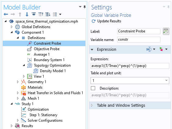
Screenshot showing the probe that defines the constraint expression.

The Optimization study step within the Study branch, which you get as part of the Optimization Module, allows us to introduce objectives, constraints, and control parameters. The objectives and constraints can be global variables, such as the probes mentioned above. Let’s look at the setup for this case.

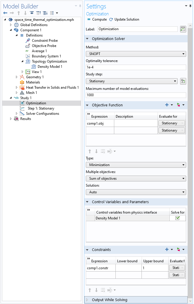
Screenshot of the Optimization study step within the Study branch, defining the Optimization solver type, the objective, the design variables, and constraints.

The screenshot above shows the Optimization study step within the Study branch. It is within this feature that we define the optimization solver, the objective function, the design variables, and the constraints. At the top of the settings, we see that the SNOPT solver is used. This solver expects that the objective function, and constraints, are differentiable with respect to the design variables. The Optimality tolerance and Maximum number of model evaluations govern how many iterations the solver will take it its attempts to find the optimum. The next three sections define the Objective Function, the Control Variables and Parameters, and the Constraints.

With the objective function, design variables, and constraints defined, it is now just a matter of solving the model.

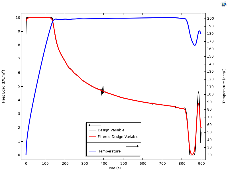
Plot of the design variable, filtered design variable, and temperature along the axis representing time.

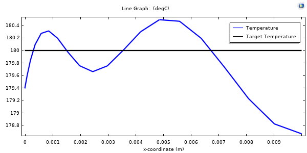
Temperature (in blue) compared to the target temperature (in black) at the final time, showing that the temperature field is very near to the target temperature over the 1D domain.

This model, which includes a material nonlinearity in the thermal conductivity, takes about a minute to optimize to the solution shown in the figures above, which plot the temperature of the heated side of the slab over time, the filtered variable and unfiltered design variable, as well as the final temperature through the cross section of the slab. It is particularly interesting to observe that the optimization solver finds a solution that leads to peak heating at the very beginning, with a heat load gradually decreasing so as not to exceed the constraint on peak temperature, and then going to zero as the temperature field equilibrates toward the optimum throughout the slab, with a final short duration increased heating to counteract the cooling to ambient. Thus, it is possible to explain the solution in a qualitative sense, but it would be difficult to get it right for a specific situation without optimization.

At this point, you might be asking yourself what the advantage of this approach is. In fact, you could just as well solve the entire optimization problem purely in the time domain, so what has been gained? Speed and simplicity.

By reformulating into space-time, we now solve a stationary optimization problem, which is faster to solve than a transient optimization problem. We can also use the built-in topology optimization features including the Helmholtz filter, thus making it very easy to set up an arbitrary, constrained, smoothed, forcing function over time. So what is the drawback, other than some conceptual complexity? This technique will use more memory. By solving in space and time simultaneously, our system matrix gets larger in proportion to the mesh along the time axis, and this mesh has to be fixed prior to the simulation. For such a 2D model, though, the memory requirements are quite modest, even with a very fine mesh.

The memory requirements for a model with two spatial dimensions do get larger, but still not exorbitantly so. An example of such a case of optimizing a 2D model with the third dimension being time is also presented via the link below and includes the Electric Currents physics in addition to heat transfer to model Joule Heating optimized over time. Otherwise, it uses the same techniques developed here. Happy modeling!

Try It Yourself

Try optimizing a heat load over time using a space-time model. Click the button below to access the model file.