
In this blog post, we explore a powerful tool in the COMSOL Multiphysics® software called state variables. We learn how they can be used to generate fractals, such as the famous Mandelbrot set and so-called fractal noise. Producing fractals is not the most typical use of state variables. Nevertheless, this blog post is an instructive, insightful, and fun way to learn more about using state variables, complex arithmetic, and random numbers.
What Are Fractals?
Broadly speaking, fractals are objects that exhibit some form of self-similarity at different scales. This may sound rather abstract, but fractal patterns actually occur in nature — You have encountered them yourself, with or without thinking about it.
Ferns, for instance, show fractal patterns. Each fern leaf shown in the figure below is composed of smaller “branches” or subdivisions, so-called pinnae, which grow along a main stem and show similar patterns as the main leaf itself. Individual pinnae are again composed of smaller subdivisions (pinnules), which in some ferns may subdivide into even smaller parts.

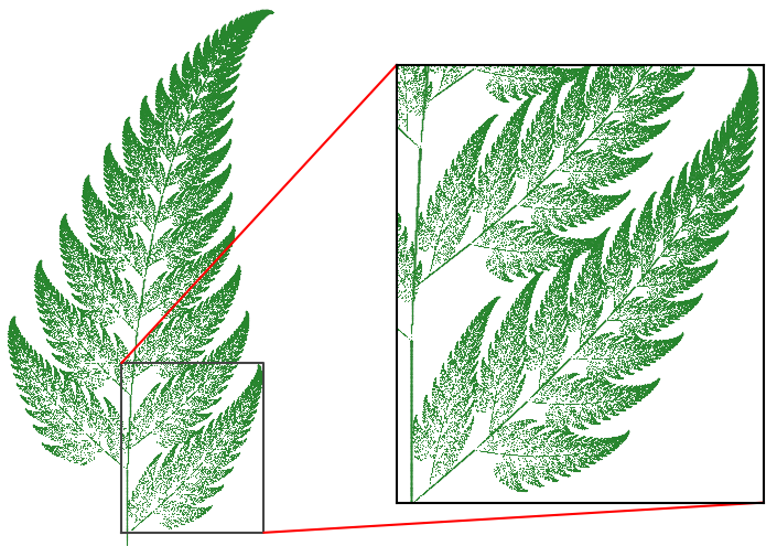
Real fern leafs and a computer-generated Barnsley fern.
There is a mathematical counterpart inspired by the pattern found in nature, namely the Barnsley fern. This mathematical representation of a fern leaf can be generated on a computer with an iterative function that requires only a few lines of code. The resulting image resembles a fern leaf that, like the real-world inspiration, is composed of subdivisions with similar shapes to the main leaf itself. In fact, the Barnsley fern will subdivide into smaller, self-similar shapes infinitely often, whereas the self-similarity in the real fern only holds for a few levels.
Besides their appealing looks, fractals actually have various real-world applications, as discussed in a previous blog post. Another application is in computer-generated imagery, like in computer games to imitate naturally looking objects such as landscapes, clouds, trees, or other plants. Later in this blog post, we will show how to generate a somewhat realistic-looking landscape using fractal patterns.
The Mandelbrot Set
Perhaps one of the most famous fractals is the Mandelbrot set. In short, it is a set of complex numbers produced by a simple iterative function. A complex number, c, is considered to be part of the set if it is plugged into a certain iterative function and the absolute value || z_\textrm{n} || does not diverge after many iterations. To check if a number is part of the set, we simply plug it into the following formula:
For example, let’s try the number c=1+0.25 i. The first iteration yields z_1=1+0.25 i (|| z_\textrm{n} ||=1.03), the second z_2=1.94+0.75 i (|| z_\textrm{n} ||=2.08), the third z_3=4.19+3.16 i (|| z_\textrm{n} ||=5.25), and so on. In this case, the absolute value || z_\textrm{n} || appears to diverge, so 1+0.25 i is not part of the Mandelbrot set.
Computing the Mandelbrot Set in COMSOL Multiphysics®
It is actually very simple to compute the Mandelbrot set in COMSOL Multiphysics. To do so, we create a 2D geometry, which we interpret as a complex plane. Each point (x,y) in this plane represents a complex number c=x+i y that we can plug into the iterative equation. We must keep track of the previous result z_\textrm{n} to compute the next number z_\textrm{n+1}.
When we are faced with the situation of keeping track of data from a previous computation step, the State Variables feature is a convenient tool. In the State Variable feature, we can define as many variables as needed. In this case, we define two variables, namely zn and aura.
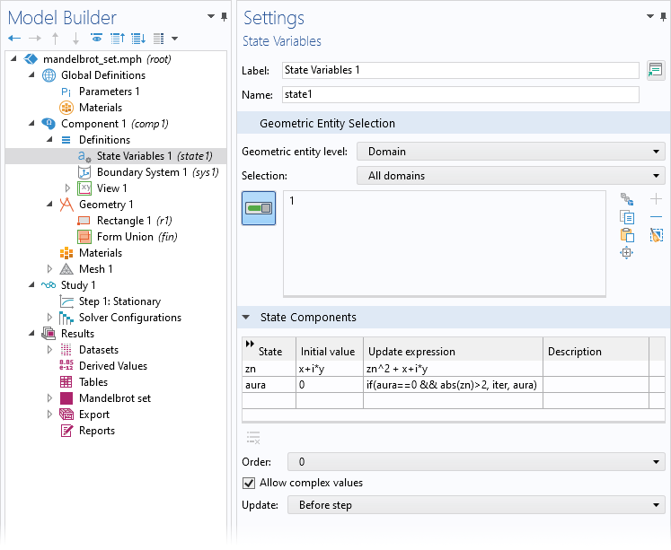
Definition of the state variables.
The first state variable keeps track of the current value of z_\textrm{n} at any given iteration step and for any given point in our complex plane. We initialize zn in the Initial value column. The Update expression is our iterative function, where we square the result zn from the previous iteration and then add c=x+i y. We have also added a second state variable called aura. We initialize the field with zero, and we store the number of iterations required until the absolute value of zn is greater than two.
It can be shown that z_\textrm{n} will eventually diverge if || z_\textrm{n} || > 2 during some iteration step. If we solve these functions for a couple of iterations and plot the result, we will see the Mandelbrot set emerging.
The Mandelbrot set and its “aura” computed for 25 iterations.
The black-gray shape represents the complex numbers that are part of the Mandelbrot set (variable zn). With each iteration, we get a closer approximation of the numbers that are actually part of the set. The different shades of gray indicate the absolute value of zn. For some initial values, c, the iterative function does not converge to a single value, but instead it jumps between different values, which in the animation, look a bit like light sources being turned on and off again. The colorized field outside of the Mandelbrot set represents the aura, which indicates how fast the numbers diverge. The closer we get to the boundary of the Mandelbrot set, the more iterations are required before the absolute value is greater than two.
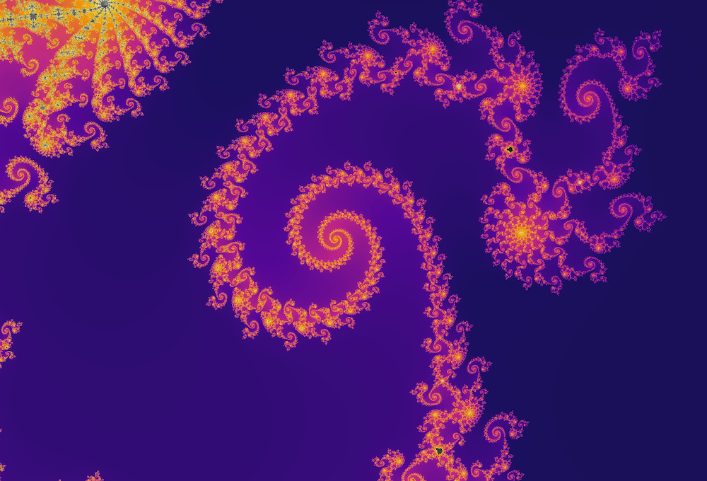
Spiral structures at a center location of c \approx -0.7789333 + 0.1345 \, i computed using 300 iterations. The image spans a width of 0.01 and a height of 0.00666.
Fractal Noise
Now that we get the gist of fractals and state variables, let’s have a look at a more practical application of fractals in the field of computer-generated imagery. More specifically, we will have a look at how so-called fractal noise can be used to emulate organic-looking textures. This technique is actually used in COMSOL Multiphysics to achieve realistic visualizations of various materials, as we will discuss later. Another common application of fractal noise is in computer games to procedurally generate natural-looking terrains.
Let’s create an artificial landscape using noise. In the context discussed here, we understand noise to be some random values. In other words, we are looking for a function, say noise(x, y), which takes two coordinates as arguments and returns a pseudorandom number. The result is interpreted as the height of the terrain at the given position. With the Random function in COMSOL Multiphysics, we can create so-called white noise. If we plot the results in the xy-plane, the numbers jump randomly and independently from one coordinate to the next increment. Obviously, this does not look like any landscapes found in the real world, so we need a better approach.
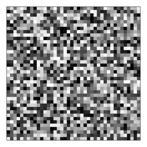
White noise with a uniform distribution. Values jump randomly between some minimum and maximum value.
Perlin Noise
Instead, we are looking for a noise function that produces random values, which at the same time, should not be “too random” and rather natural looking. There should be some coherence between neighboring points. Perlin noise, developed by Ken Perlin, is a special form of noise that allows us to produce pseudorandom values for given coordinates, and the transition of the noise value from one point to a neighboring point is smooth. This “smooth randomness” looks more like patterns found in nature.
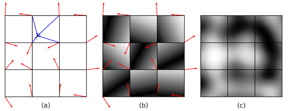
Generating 2D Perlin noise: (a) Grid definition. The red arrows are randomly generated gradient vectors (scaled by 0.5 for better visualization). The blue arrows point from the surrounding grid points to some position (x, y). (b) Absolute value of the first dot product using the bottom-left gradient vector. The gray scale indicates values between 0 (black) and 1 (white). (c) Interpolated noise.
Generating Perlin noise involves a few steps, outlined above. In the first step, we divide our xy-plane into a grid of unit squares. At each grid point, we generate a pseudorandom vector of length one, which is also referred to as a gradient vector (red arrows). The four surrounding gradient vectors associated with a point (x,y) are only pseudorandom, since they should always be the same when we recompute the noise at the same point. With the gradient vectors, we can start to compute the noise value for some point (x,y) located anywhere inside the plane. For this given point, we compute four dot products between the gradient vectors, and the position vectors pointing from a grid points to the chosen point (x,y) itself (blue arrows).
The four dot products can be interpreted as the influences that the gradients have onto the noise level at the chosen point. The dot product between the gradient vector, \mathbf g_\textrm{i}, and the position vector, \mathbf x – \mathbf x_\textrm{gi}, attains its maximum value when both vectors point in the same direction, and its minimal value when they are perpendicular to each other. The final step in generating Perlin noise is to compute a weighted average of the four dot products and to return the interpolated value. This involves a cleverly chosen smoothed step function and linear interpolation, which makes sure that we get smooth transitions over our domain. More details on how to compute Perlin noise can be found in Ref. 1.
Fractal Noise
The Perlin noise we generated has very smooth transitions, and it does perhaps not look like most real-world terrain would, where we typically find more local irregularities, perhaps from hills or smaller rocks. The solution is to superpose different octaves of noise, and this is where the idea of fractals comes into play. Basically, we generate more noise with higher frequencies, or in other words, with more peaks and valleys over the same distance. Like in music, the frequency is doubled with every octave. We decrease the amplitude of the higher-frequency noise and add it to the base noise. In principle, we can add as many octaves of noise as we like. So, instead of calling the noise() function only once, we now call it multiple times and sum the results with the adjusted amplitudes.
If we interpret h as the height of our landscape, the first iteration (j=0) yields a first, smooth approximation of the terrain with large, defining features such as mountains; the second iteration might be from more local hills and depressions; the third iteration might be from individual boulders and rock formations; and so on.
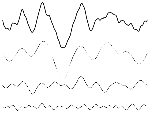
1D fractal noise (top line). Below are the first three frequencies of Perlin noise, which when added together, form the line at the top.
Producing fractal noise involves computing and superposing noise with different frequencies. When doing this in COMSOL Multiphysics, it is again convenient to make use of state variables, since we want to “remember” the combined noise from all previous frequencies. The following animation represents a 2D height map, where more and more details in the terrain emerge with each level of higher-frequency noise, which is added to the base noise.
Terrain map generated by superposing five frequencies of Perlin noise. The contour lines and the different colors represent different heights.
Randomized surface geometries can be used in physics simulation contexts where, for example, you need to model surface roughness or inhomogeneous materials. In previous blog posts, we showed a different way to create random surface geometries by superposing trigonometric functions with varying amplitudes and frequencies, as well as methods to create arbitrary geometries from image or text files.
Improving Material Appearance by Using Noise
Did you know that you can add fractal noise to your plots to improve material appearances in COMSOL Multiphysics? As of version 5.6, there are special visualization options for materials. Some built-in material types, such as rusty steel, leather, and water, use Simplex noise to create more realistic-looking textures. Simplex noise has similarities to Perlin noise and was also developed by Ken Perlin. You may tweak the noise parameters yourself to achieve the effect you want.
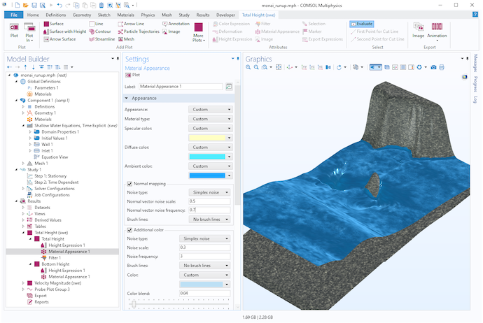
Visualization of water using Simplex noise in a shallow water equation model.

Visualization of a wrench model with a rusty steel surface using Simplex noise.
Try It Yourself
Want to try modeling the Mandelbrot set or Perlin noise discussed in this blog post? Click the button below to access the MPH files.
Reference
- K. Perlin, “Improving Noise”, New York University, 2002. https://mrl.cs.nyu.edu/~perlin/paper445.pdf.
Further Reading
Learn more about fractals, noise, and state variables in these related blog posts:


Comments (0)