
The B-H curve is generally used to describe the nonlinear behavior of magnetization that a ferromagnetic material obtains in response to an applied magnetic field. In this blog post, we will show you how the B-H curve affects your magnetic analysis and how to improve it, using a demo application available as of version 5.5 of the COMSOL Multiphysics® software.
The B-H Curve, Permeability, and Differential Permeability
Magnetic soft iron steels are widely used as core materials in motors, transformers, and inductors. If they are placed in a region without magnetic fields, they will remain without a magnetic field; they do not have an “intrinsic” magnetization. The B-H curve is usually used to describe the magnetization properties of such materials by characterizing the permeability \mu, which is defined as:
where \mathbf{B} and \mathbf{H} represent the magnetic flux density in tesla (T) and the magnetic field intensity in ampère per meter (A/m), respectively.
COMSOL Multiphysics has more than 200 built-in materials with B-H curves. Specifically, the Nonlinear Magnetic material library covers most of the widely used nonlinear magnetic materials. COMSOL Multiphysics usually uses an interpolation function with a local table to define the B-H curve. You can also plug in your own B-H curves by adding the B-H Curve material property to a new magnetic material.
The B-H curve of a material can be measured in the laboratory by following standards and procedures. However, it is difficult to perform a direct measurement when \mathbf{B} is above the saturation induction, which is referred to as the overfluxed region. Generally, it is difficult for test equipment to reach such a high level of stable \mathbf{B}; for instance, 1.8 T. Even if the test equipment can do so, the measured data will typically be inaccurate due to the test frame getting overheated. For this reason, the B-H curve data in the overfluxed region is usually obtained using extrapolation methods; for example, the simultaneous exponential extrapolation (SEE) method (Ref. 1).
From the numerical point of view, the slope of the B-H curve is of great importance, since the nonlinear iterative solver uses it to evaluate the local linearization of the nonlinear material behavior. Thus, it is more useful to consider the differential permeability or the incremental permeability, especially for nonlinear magnetic materials. The differential permeability is defined as:
For standard materials, \mu_D is larger than 0, which implies that the B-H curve is monotonically increasing. For ferromagnetic materials, \mu_D decreases to the permeability of vacuum \mu_0 after magnetic saturation, as illustrated in the figure below.

The schematic diagram of a typical B-H curve and the corresponding differential permeability as a function of magnetic field intensity.
How the Extrapolation of the B-H Curve Affects the Simulation
In the Settings window of the B-H Curve interpolation function, you can click the Plot button to visualize the B-H curve. For a better visualization, the Extrapolation can be set to Constant. However, this setting is not recommended for the study, since otherwise, the B-H curve will have discontinuities at the start and end points of the B-H curve data.
To understand how the setting actually affects the simulation, let us take the E-Core Transformer tutorial model in the AC/DC Module Application Library as an example. It takes about two minutes when setting the B-H curve extrapolation to Constant and one minute when setting it to Linear for a time-dependent study from 0 to 0.05 s. The convergence plots of the two simulations explain the difference in computation time. As the figure below indicates, due to the discontinuities caused by the Extrapolation setting, it requires much smaller time steps to find a solution when the magnetization reaches saturation.
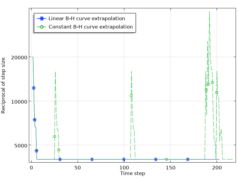
The convergence plot of the simulation with a linear and constant B-H curve extrapolation.
How the Smoothness of the B-H Curve Affects the Simulation
In addition to the issues of the extrapolation, the \mu_D curve from measured B-H data may contain ripples that are generally unphysical. Such unphysical ripples cause numerical instabilities that result in longer computation times or even a lack of convergence. Take the E-Core Transformer model as an example again. The model uses the built-in Soft Iron material where the B-H curve is smooth. Now, we change the curve by modifying a few data points to make three new groups of B-H curves, as shown below. Let’s run the time-dependent study in the model with these three B-H curves and all of the other settings the same. The simulation details are listed in the table below, and the convergence plots are shown in the figure below.
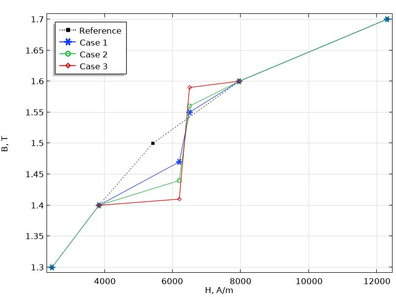
The plot of three groups of B-H curves with the reference from the built-in B-H curve. Note that the plot only shows a part of the curve where the differences take place.
| Case |
B-H Curve Data
H (A/m), B (T) |
Computation Time |
|---|---|---|
| 1 |
… 3841.67, 1.4 6200, 1.47 6500, 1.55 7957.75, 1.6 … |
1 minute, 17 seconds |
| 2 |
… 3841.67, 1.4 6200, 1.44 6500, 1.56 7957.75, 1.6 … |
1 minute, 45 seconds |
| 3 |
… 3841.67, 1.4 6200, 1.42 6500, 1.58 7957.75, 1.6 … |
Nonlinear solver did not converge. Maximum number of Newton iterations reached. Time: 0.029466491699218753 seconds. Last time step is not converged. |
B-H curve data and computation times for the three cases.
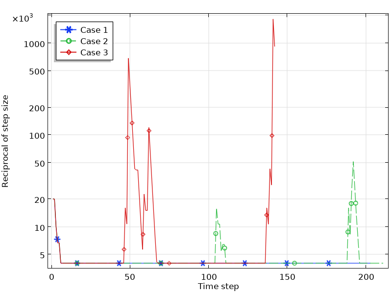
The convergence plot of the simulations for the three cases.
As can be seen from these figures, the smoothness of the B-H curve affects the simulation results significantly. For Case 1, where the B-H curve data deviates from the reference slightly, the simulation runs smoothly. For Case 2, where the change of the B-H curve slope increases to some degree, the simulation is still converged, but requires a much longer simulation time. As the slope change increases further, the simulation even fails to converge (Case 3).
Optimize the B-H Curve with the Click of a Button
As of COMSOL Multiphysics® version 5.5, the B-H Curve Checker application is available. This simulation application can be used to check and optimize the B-H curve measured from experiments. The application can generate the curve data in the overfluxed region where measurements would be difficult. The application can also remove the unphysical ripples of the slope of the B-H curve that might cause numerical instability.
The application evaluates the original B-H curve from two aspects:
- If the extrapolation of the curve is reasonable from the physical point of view
- If the slope of the curve is smooth
The optimization algorithms are mainly based on the simultaneous exponential extrapolation method and the linear interpolation method, respectively.
The application requires the original curve data defined in a text file as the input. Once the curve is imported, the application will check if it requires optimization. By clicking the Optimize button, the application user can generate the optimized curve data, which can be exported to a text file.
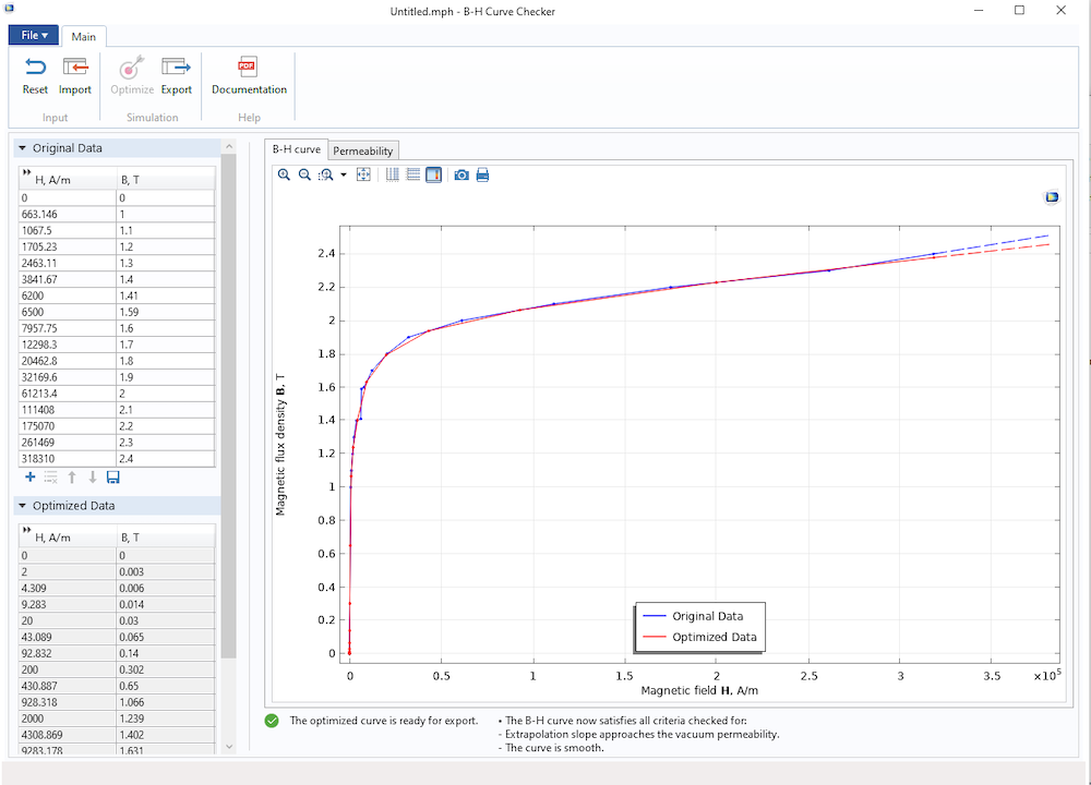
The B-H Curve Checker application, showing the original and optimized B-H curves.
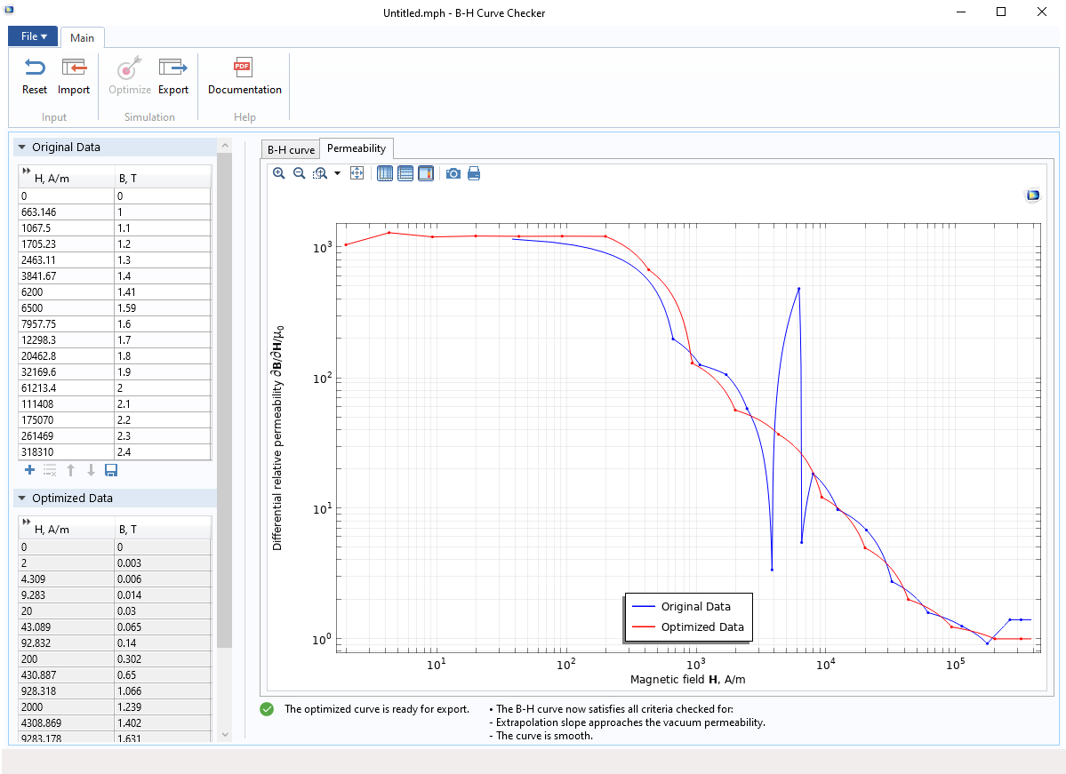
The B-H Curve Checker application, showing the differential relative permeability of the original and optimized B-H curves.
Optimized Nonlinear B-H Curves in the Material Library
The B-H Curve Checker application has been applied to the built-in materials, out of which 35 are optimized for increased performance and stability. The list of corrected materials is given as follows:
- AC/DC Module material library
- Soft Iron (Without Losses), B-H curve and Effective B-H curve
- Soft Iron (With Losses), B-H curve and Effective B-H curve
- Nonlinear Permanent Magnet, B-H curve
- Nonlinear magnetic material library
- Silicon Steel NGO 35JN200
- Silicon Steel NGO 35PN210
- Silicon Steel NGO 35PN230
- Silicon Steel NGO 35PN250
- Silicon Steel NGO 50PN1300
- Silicon Steel NGO 50PN600
- Silicon Steel NGO 50PN700
- Silicon Steel NGO 50PN800
- Silicon Steel NGO M-22
- Silicon Steel GO 3%
- Silicon Steel GO 3413
- Silicon Steel GO 3423
- Silicon Steel GO Silectron 4 mil cross
- Silicon Steel GO Silectron 4 mil rolling
- Metglas Nano Finemet 50 Hz NoFieldAnnealed
- Cobalt Steel Vacoflux 50
- Nickel Steel 4750
- Nickel Steel Monimax Nonoriented
- Nickel Steel Mumetal 80% Ni
- Nickel Steel Square 50
- Nickel Steel Superperm 49
- Low Carbon Steel 50H470
- Low Carbon Steel Magnetite
- Low Carbon Steel Soft Iron
- Low Carbon Steel Vacofer S1 Pure Iron
- Alloy Powder Core Hiflux 125 mu
- Alloy Powder Core Hiflux 160mu
- Alloy Powder Core Koolmu 125 mu
- Alloy Powder Core Koolmu 40 mu
- Alloy Powder Core Koolmu 75 mu
- Alloy Powder Core Koolmu 90 mu
- Alloy Powder Core MPP 60 mu
Note that materials added to a model prior to COMSOL Multiphysics® version 5.5 are not affected, unless reloaded from the material library.
Frequency Study for Soft Iron Materials
The B-H curve is usually nonlinear, and it can be used in the stationary and time-dependent studies. However, it cannot be used directly in frequency-domain studies. To solve in the frequency domain, you would need a “cycled averaged” B-H curve that approximates a nonlinear material at the fundamental frequency. For more information, please read our previous blog post: Model Magnetic Materials in the Frequency Domain with an App.
Summary
In this blog post, we introduced the widely used B-H curve and its important properties for modeling soft iron materials. We also demonstrated how the settings of the extrapolation and the smoothness of the curve could affect your magnetic simulations with case studies.
We then introduced the new application released in COMSOL Multiphysics® version 5.5, the B-H Curve Checker. The application could be used to optimize the measured B-H curve with the click of a button after importing the curve. We also introduced the improvement of all of the B-H curves in the nonlinear magnetic material library. Finally, we mentioned that you could use another application, the Effective Nonlinear Magnetic Curves Calculator, to compute effective B-H curves for frequency-domain studies.
Related Reading
Learn more about modeling magnetic materials on the COMSOL Blog:
- Modeling Ferromagnetic Materials in COMSOL Multiphysics®
- Evaluating Transformer Designs with Electromagnetics Simulation
- Model Magnetic Materials in the Frequency Domain with an App
Reference
- D.K. Rao and V. Kuptsov, “Effective Use of Magnetization Data in the Design of Electric Machines With Overfluxed Regions”, IEEE Transactions on Magnetics, vol. 51, no. 7, pp. 1–9, 2015.


Comments (8)
Mudan Chen
August 11, 2020Hi, where is the optimise button?
Lipeng Liu
August 11, 2020 COMSOL EmployeeHello Mudan,
Thank you for your comment.
If you did not see the button as shown in the screenshot, please contact our Support team.
Online Support Center: https://www.comsol.com/support
Email: support@comsol.com
Ben Godlun
April 28, 2022Hi, i’m using the material “Alloy Powder Core Ferrite R 2300 mu” it has a BH Curve interpolation that uses a ‘local table’ data. I wish to know at what temperature and frequency is this data measured.
Lipeng Liu
April 28, 2022 COMSOL EmployeeHi Ben,
The material you used are from a third party (BHmag Database, supplied by Precision
Wafers Inc. Copyright © 2013 by Precision Wafers Inc.). For more information, please check with them.
Regards,
Lipeng
Sergio Pesenti
May 5, 2022Hey Lipeng,
I am interested in the Silicon Steel NGO materials of the library.
I would like to compare the BH curves in the COMSOL library with real data from steel suppliers.
Where did you find these data to build the tables?
Lipeng Liu
May 6, 2022 COMSOL EmployeeHi Sergio,
1. Add the material to a model, such as Silicon Steel NGO 35PN270.
2. Go to Component->Materials->Silicon Steel NGO 35PN270->B-H Curve->Interpolation,
3. You will find the table in the Settings window.
Regards,
Lipeng
Gabriel Barroso De María
March 16, 2025Hello,
thanks for this interesting post.
Would it be possible to model the H variations in AC, with complex permeability around a working point close to saturation of the B-H curve?
Thanks in advance
Best regards
Lipeng Liu
March 17, 2025 COMSOL EmployeeHi Gabriel,
Yes. Please provide more details and our support will help you.
Online Support Center: https://www.comsol.com/support
Email: support@comsol.com
Regards,
Lipeng