How to Convert Point Cloud Data to Surfaces and Solids

Not all analysis projects start with a CAD model. Sometimes the only data you have available is a set of points, also known as a point cloud. In this blog post, we will show how point cloud data can be converted to geometry models that can be used for simulation in the COMSOL Multiphysics® software.

What Is a Point Cloud?

A point cloud is a set of points in 3D given by x-, y-, and z-coordinates. The points typically originate from the surface of a physical object that has been scanned using a laser, metrology tools, radar, etc.

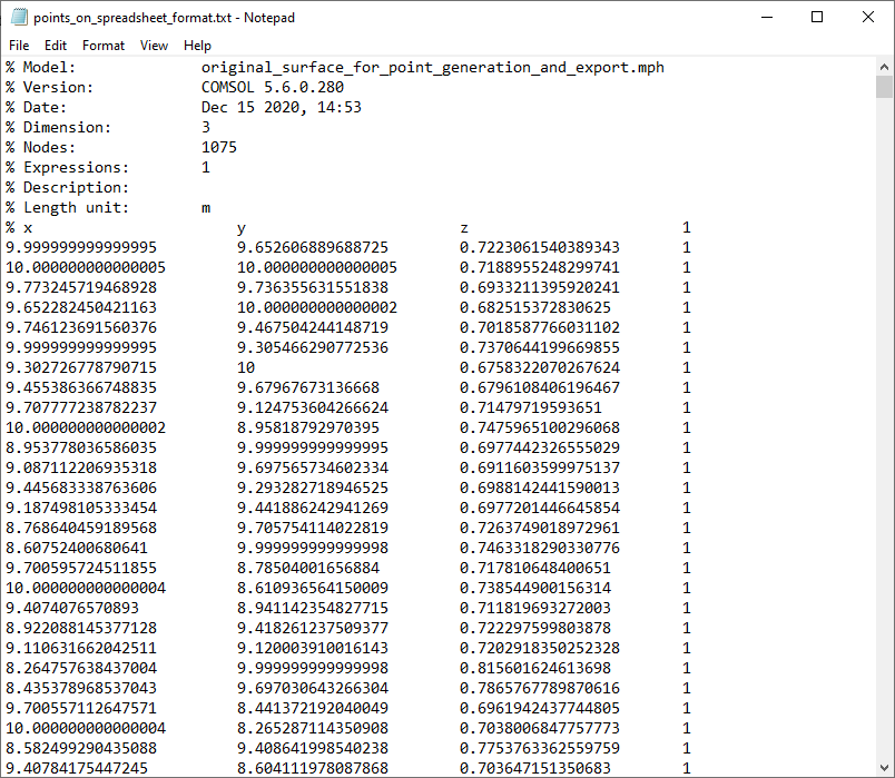
The screenshot below of a text file in Notepad shows the beginning of a point cloud data file with x-, y-, and z-coordinates organized in tab-separated columns.

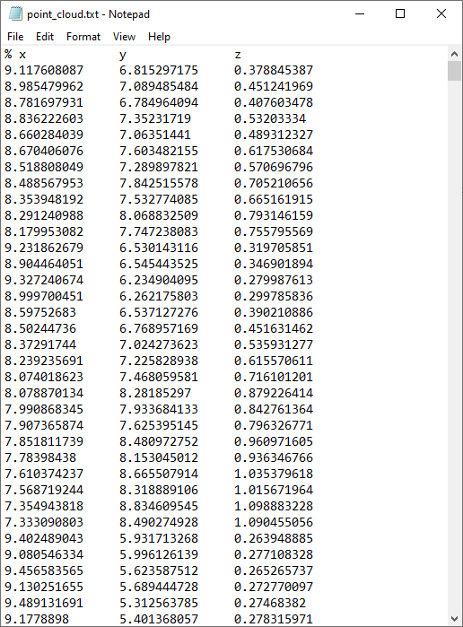
A text file with point cloud data.

This is one of the simplest types of coordinate formats that COMSOL Multiphysics can import. In the software, it is called the Spreadsheet format. In this format, you can use an optional % (percent) character to indicate a comment line. Values and indices can be separated by space, comma, semicolon, or tab characters.

Once imported, a point is assigned an index according to the line number in the file for its coordinates. There are often ambiguities in such a point set, since there is no information about the relationship between the points, also known as connectivity. To illustrate the type of ambiguity that may occur, let’s look at a simple 2D example. Consider the 2D curve in the figure below. From the figure, it is obvious that the points 5, 18, and 7 are consecutive points on the curve.

However, in the next figure, which corresponds to the curve represented by imported point cloud data, this is not so obvious. Perhaps 5, 6, and 4 are consecutive points on the curve?

Point cloud data may have intrinsic ambiguities. Are points 5, 6, and 4 connected? In this case they are not connected, which can be seen from the original curve, but not from its relatively sparsely sampled point cloud.

If an imported list of 3D coordinates comes with associated triangulated surface connectivity data, such as for the STL, PLY, or 3MF file formats, then this ambiguity is resolved. We then have a list of triangles defined by the connectivity between points, which uniquely defines the surface. For example, in a surface triangle data file, a row such as

15 17 23

would mean that points with indices 15, 17, and 23 are connected as the vertices in a triangle.

On the other hand, if all we have is point cloud data without connectivity information, then in order to resolve such ambiguities, we need to make additional assumptions. One such assumption can be that the surface data is of the form z=f(x,y), also known as a function surface. If the data is not on that form, we can always try to break it up into several pieces, each on the form z=f(x,y). Note that data on the form y=f(x,z) or x=f(y,z) would be equally useful after some rearrangements.

Visualizing the Point Cloud

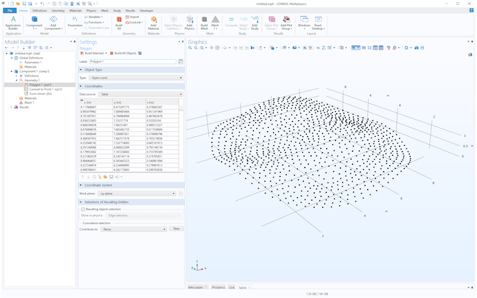
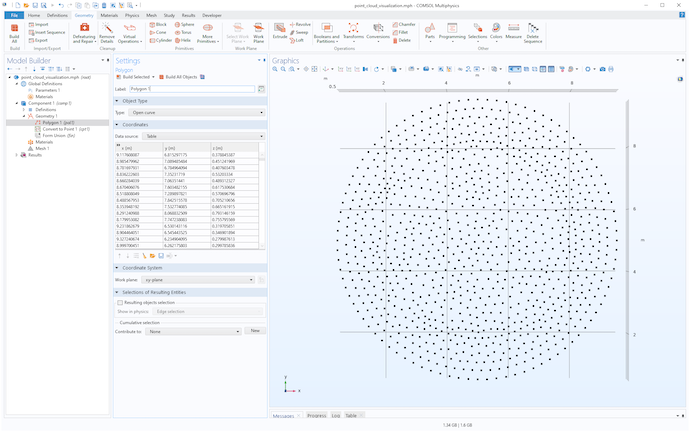
One easy way to visualize point coordinate data is to import it as a table to a Polygon geometry object and then use a Convert to Point operation, as shown in the figures below.

A visualization of the point cloud data as geometry point objects seen from two different viewing angles.

Based on this visualization, we can assume that the point cloud defines a function surface of the form z=f(x,y). For later use, we will need to know the extents of the point cloud. An easy way to get this information is to right-click the Geometry node and select Measure.

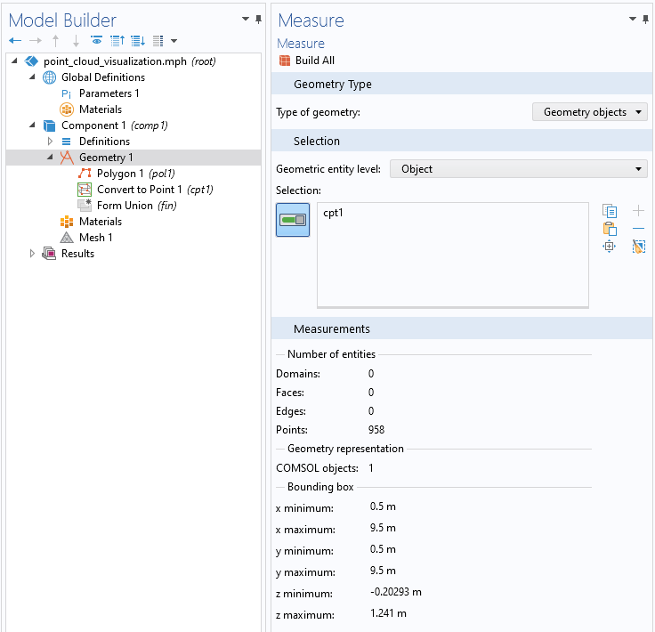
The Measure Settings window gives us information about the extent of the point cloud.

We can see that there are 958 points extending from 0.5 to 9.5 in both the x– and y directions, and from about -0.2 to +1.5 m in the z direction. The unit used in this example is meter (m).

We can now try to convert this set of points to a surface by using the operation Convert to Surface. However, this doesn’t work. It will give us an error message, since we don’t have the connectivity information for the points. We need to somehow construct the connectivity data. In addition, we need to use the assumption that data is on the form z=f(x,y). The solution is to import the point cloud as an unstructured interpolation surface.

Creating an Interpolation Surface

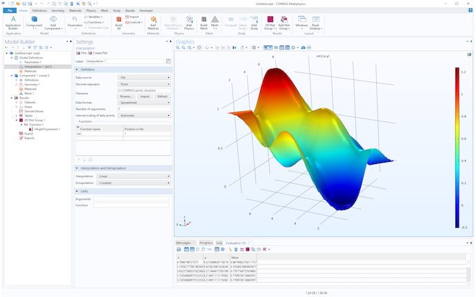
As a next step, we add an Interpolation function under Global Definitions and set the Data source to File. Browse to the point cloud text file, in this example, C:\COMSOL\point_cloud.txt, as shown in the figure below. You can download this file from the link at the end of this blog post.

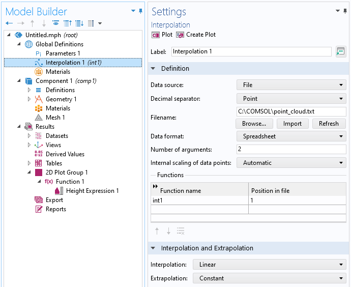
The Interpolation function defined by the point cloud.

The Interpolation functionality will automatically guess that the data is on the form z=f(x,y) and that the first two columns in the file represent the x– and y-coordinates, respectively, and that the third column represents the function value, which we will interpret as the z-coordinate of a function surface. You can see this from the number of arguments, which is automatically set to 2, corresponding to the x– and y-coordinates, respectively. The Function name is automatically set to int1 (you can change this) and the Position in file setting 1 means that the function value for int1(x,y), representing the z-coordinate, will be given by the first column following the input argument columns. In other words, column number 2 + 1 = 3. In this case, the file only has three columns, so 1 is the only choice. If the data is on a different form, you can use a text editor or spreadsheet software, such as Excel®, to rearrange the data before importing.

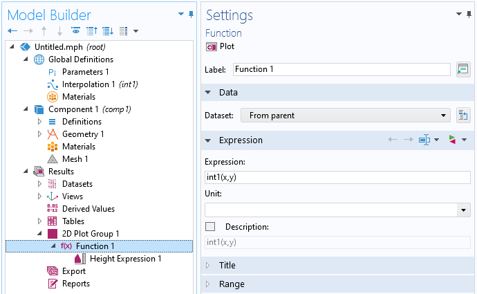
Now, click the Plot or Create Plot button, located at the top of the Interpolation Settings window, to visualize the interpolation function. The Plot option will create a temporary visualization, whereas Create Plot will create a 2D Grid dataset and an associated Function plot in a 2D Plot Group under Results.

A visualization of the interpolation function as a Function plot under Results and its associated Settings window.

How did the software create this surface representation based solely on the assumption z=f(x,y)? The interpolation functionality creates, behind the scenes, a 2D triangulated mesh of the x– and y-coordinates, then associates the function values to each point, and finally performs a linear interpolation between the function values. You can think of it as dropping a fishnet on top of the point cloud. Note that this triangulated mesh is invisible to the user. In the Interpolation and Extrapolation section, in the Interpolation Settings window, you can see the settings for Interpolation, which is by default set to Linear. The other option is Nearest neighbor, which creates a piecewise constant function interpolation that is not useful here.

The other setting in this section is Extrapolation. This is used to guess the values of the function outside of its domain of definition, which is determined by its x– and y-coordinates. In this case, the point cloud is distributed within a circle in the xy-plane. When visualizing the data as a Function plot, the xy data is taken from a rectangular Grid 2D dataset, and the interpolation functionality will assign constant function values in a radial pattern, filling out the space between the circle and a rectangle circumscribing the point cloud data. This can be seen in the figure below, where you can discern the circular imprint from the point cloud data.

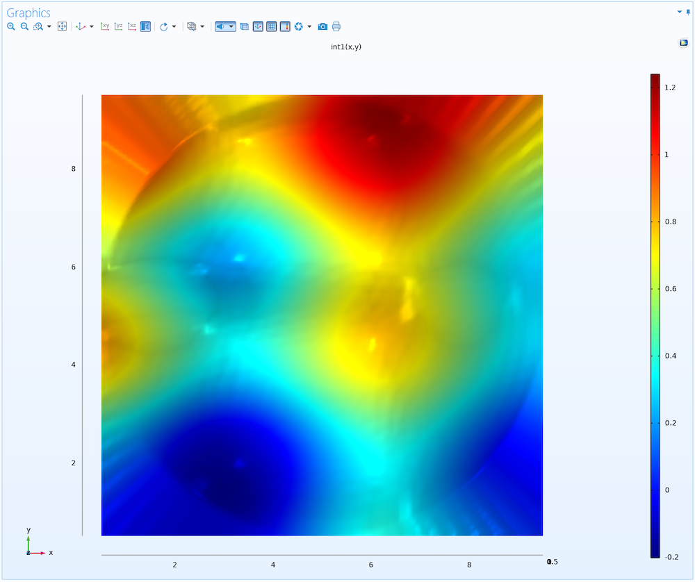
A top view of the interpolation function, where the extrapolated parts can be seen outside of the circular area that defines the footprint of the original point cloud.

How do we convert this interpolation function to a geometry representation that we can use for meshing and then simulation? This is done by using a Parametric Surface geometry object, as we will see next.

Creating a Parametric Surface

To create a geometric surface that closely follows the above interpolation function, add a Parametric Surface feature under Geometry, according to the below figure.

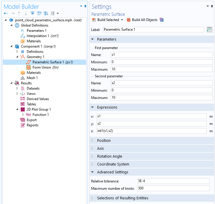
The Parametric Surface settings for the surface based on the point cloud interpolation function.

In this Settings window, we interpret s1 and s2 as the x– and y-coordinates, respectively, and int1(s1,s2) as the z-coordinate. Now, we need to use the information obtained earlier by using the Measure tool. We set the s1 and s2 minimum and maximum values to be a bit wider than the measured extents of the point cloud, to make sure we don’t miss any details.

In this case, the Parametric Surface will be defined between 0 and 10 in both directions, to be compared with the point cloud data that we measured to be between 0.5 and 9.5.

Internally, the software represents the parametric surface by a B-spline surface, which is computed to approximate the mathematical surface defined by the x-, y-, and z-expressions. A B-spline surface is a piecewise polynomial surface and the number of piecewise polynomials used is indirectly determined by the number of knots. The higher the number of knots, the higher the number of piecewise polynomials and the better the approximation can be, but at a higher computational cost. The number of knots in the B-spline surface increases automatically until the surface approximation satisfies the tolerance specified in the Relative tolerance field or until it reaches the number of knots specified in the Maximum number of knots field. The tolerance is measured relative to the space diagonal of the bounding box of the parametric surface.

In this case, trial and error leads us to 5e-4 for the Relative tolerance and 500 for the Maximum number of knots. (The default is 1e-5 and 20, respectively.) The resulting surface is shown in the following figure.

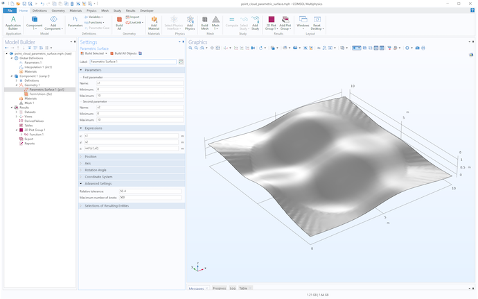
The parametric surface geometry object.

We can use the technique from earlier to simultaneously visualize the point cloud and the surface, as shown in the figure below.

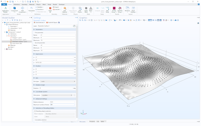
The parametric surface geometry object and point cloud.

To get more control over the level of detail of the surface visualization, you can click the Mesh node and create a mesh with a suitable Element size. The following figure shows a mesh using the Extremely fine setting. To get an even higher resolution, select the User-controlled mesh option and set a Custom element size.

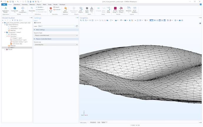
The point cloud and parametric surface geometry visualized using a mesh.

Trimming the Surface

The original point cloud data has a circular footprint centered at x = 5, y = 5 with radius 4.5. The following figure shows the result of adding a cylinder fitted to these measures and with a height that covers the minimum and maximum values in the z direction.

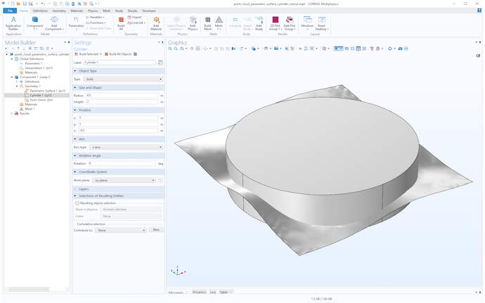
A cylinder used to trim the surface.

Now, use an Intersection operation to trim the surface by selecting both the surface and the cylinder, as shown in the figure below.

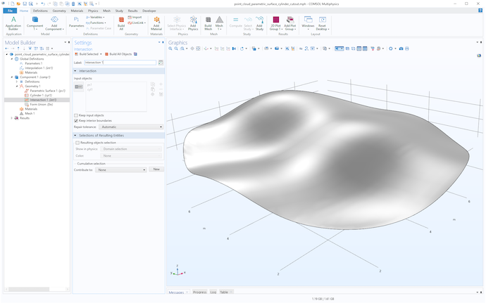
The result of intersecting the surface with the cylinder.

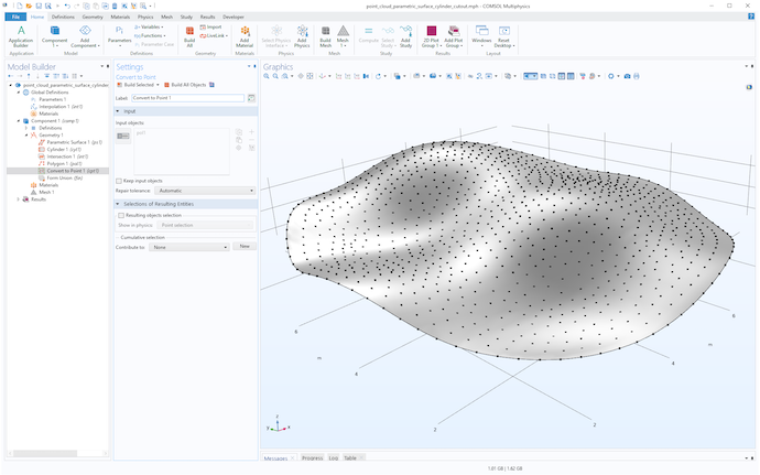
The point cloud and trimmed surface.

Creating a Solid in the Space Between Two Surfaces

To create a solid with a circular footprint in the space between two interpolated surfaces, simply repeat the above steps to import a second surface, as shown in the following figure.

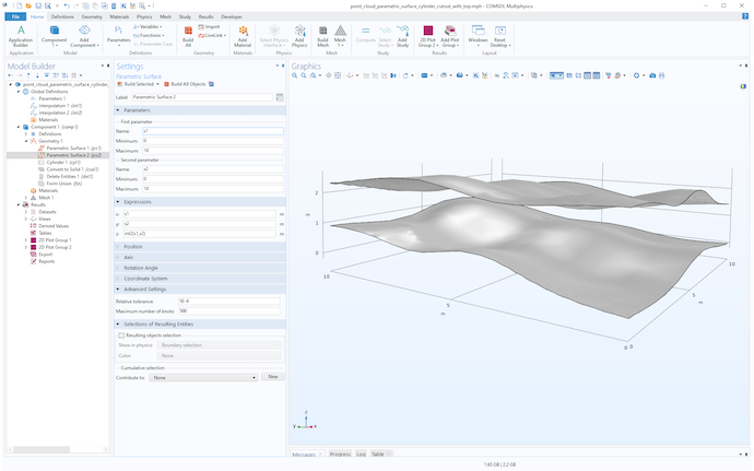
A second surface corresponding to a second point cloud.

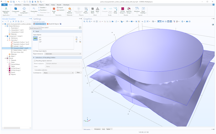
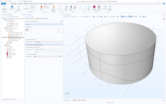
Then, create a cylinder for trimming the surfaces and use the Convert to Solid operation on all objects, as shown in the following figures.

Using a cylinder to trim two surfaces.

You can obtain the same result by using either the Partition Objects or Partition Domains operation. These operations are more sophisticated than Convert to Solid and allow you to select the cylinder as the object or domain to be partitioned. Then you can select the interpolation surfaces as the tool objects used for partitioning. The Partition Domain operation can be more versatile in some situations, since it allows you to partition selected domains from an object, and it has an option to automatically extend planar, cylindrical, or spherical tool faces when these do not intersect the domain to be partitioned.

Finally, use Delete Entities to remove the unwanted domains, as shown in the figure below.

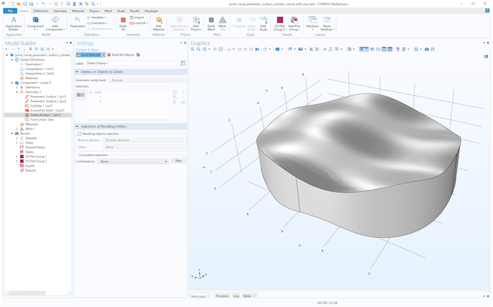
A solid resulting from importing and trimming two interpolation surfaces.

This solid can now be meshed and used for any type of simulation. In this case, we can create a swept hex-only mesh, as shown in the next figure.

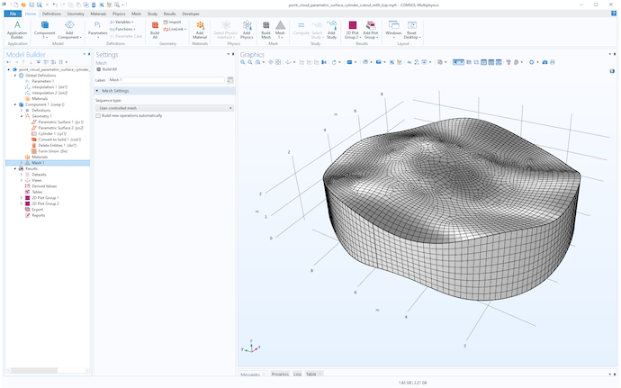
A swept mesh for the cylindrical solid.

Generating Point Cloud Data for Testing

You can download the point cloud data and files used in this blog post by following the link at the bottom of this page. If you instead would like to generate your own point cloud data, you can start from any surface. In the following figure, a parametric surface is used, trimmed with a cylinder just as in the above example, and the expression used for the z-coordinate is:

z=0.25*cos(s1)+0.2*cos(1.5*s2)*exp(-0.1*s1+0.1*0.25*s2)+0.1*s2

As a matter of fact, this is the surface that was used to generate the point cloud data used in the first example.

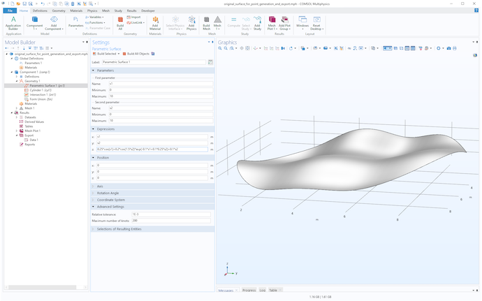
A parametric surface given by a mathematical expression and trimmed by a cylinder object.

Now, create a Mesh, then right-click the Mesh node and select Plot to generate a Mesh Plot under Results. Next, right-click Mesh Plot > Mesh and select Add Plot Data to Export. In the Settings window for Data, use 1 as the Expression. This exported constant value will not be used. Choose a Filename and click Export at the top of the window to write the data to file.

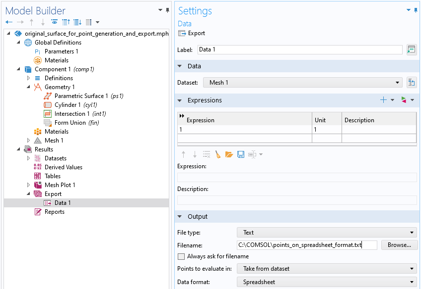
The Export settings used to export data on the Spreadsheet format.

If you open the resulting text file in a text editor or spreadsheet software, you will see a header with comment lines and four columns. The last column contains the constant Expression 1.

In a spreadsheet software, such as Excel®, you can delete column 4 and save the file again to a text file format. The resulting file will be in the same format as the examples discussed earlier. Note that the leading comment lines in the header are optional and can be removed.

Generalizations and Further Reading

The techniques above can be generalized in a number of ways. You can, for example, import more than two surfaces to create a more complicated structure. You can trim the data with an object that is not a cylinder. In other cases, the point cloud data may be based on cylindrical or spherical coordinates. You can combine the above techniques together with coordinate transformations to generate cylindrical or spherical patches.

For a real-world example of using interpolated data in a geotechnical application, see this blog post: Integration of Geological Structures into Regional-Scale Groundwater Models

For even more related examples, see this blog post: How to Build Geometries from Elevation Data to Model Irregular Shapes

Try It Yourself: Convert Point Cloud Data

Download the MPH-files and data files used in this blog post by clicking the button below. You will also find an MPH-file demonstrating how to compare the original parametric surface, defined by an expression, with the parametric surface defined by the point cloud.

Microsoft and Excel are either registered trademarks or trademarks of Microsoft Corporation in the United States and/or other countries.