How to Obtain Fatigue Model Parameters

When simulating fatigue, you are faced with two main challenges. The first is to select a suitable fatigue model for your application and the second is to obtain the material data for the selected model. I recently addressed the first challenge in the blog post “Which Fatigue Model Should I Choose?“. Today, I will address the second challenge and discuss how you can obtain fatigue model parameters.

Predict Fatigue Using Many Different Models

Fatigue models are based on physical assumptions and are therefore said to be phenomenological. Since different micromechanical mechanisms govern fatigue under various conditions, many analytical and numerical relations are needed to cover the full spectrum of fatigue. These models, in turn, require dedicated material parameters.

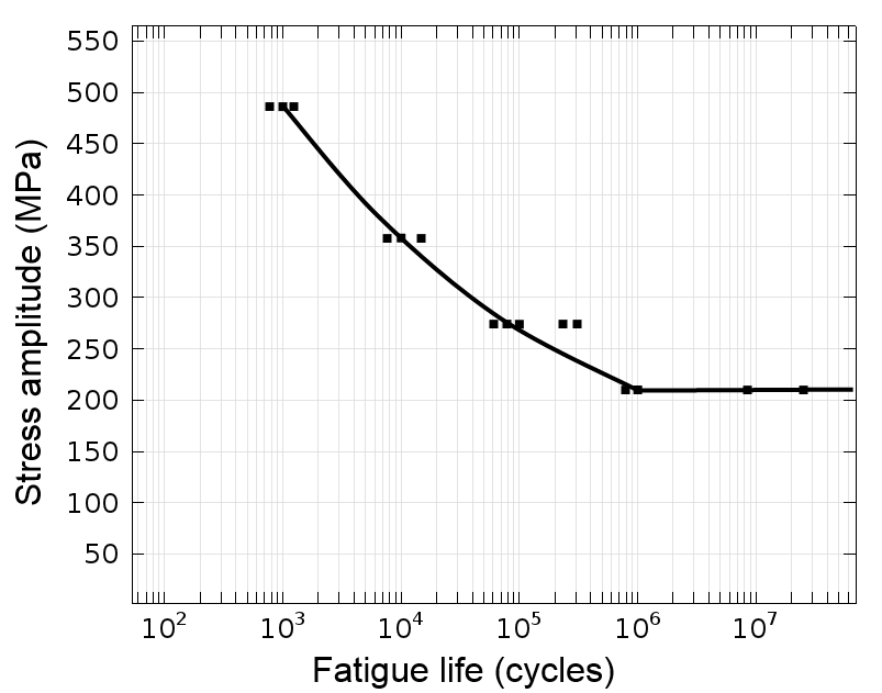
It is well known that fatigue testing is expensive. Many test specimens are necessary since the impurities responsible for fatigue initiation are randomly distributed in the material. The difference in the fatigue life is clearly visible when you visualize all the test results in an S-N curve.

An S-N curve. The black squares represent individual fatigue tests.

Advice for Obtaining Model Parameters via the S-N Curve

Since the S-N curve — also called the Wöhler curve — is one of the oldest tools for fatigue prediction, there is a good chance that the material data is already available in this form. Many times, the data is given for a 50% failure risk. If you do not have access to the material data, you are faced with a testing campaign.

When you are done, pay attention to the statistical aspect and, at each load level, select the same reliability when constructing an S-N curve. This is important since the S-N curve is expressed in a logarithmic scale where a small difference in input has a large influence on the output. Then, S-N curves for different reliability levels fall under each other and you should select an appropriate level for your application. For noncritical structures, a failure rate of 50% might be acceptable. However, for critical structures, a significantly lower failure rate should be chosen.

Always pay attention when you combine fatigue data from different sources. Make sure that the testing conditions and the operating conditions are the same.

Advice for Running Fatigue Tests that Consider Mean Stress

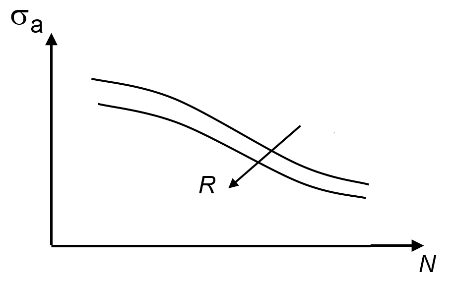
Another aspect of fatigue testing considers the mean stress that has a substantial influence on the fatigue life. In general, fatigue tests performed at tensile mean stress will give a shorter life than tests performed at a compressive mean stress. This effect is also frequently expressed using the R-value (the ratio between the minimum and maximum stress in the load cycle). Thus, with decreasing mean stress (or R-value), the fatigue life increases.

In the Fatigue Module, the Stress-Life models do not take into account this effect. When using these models, you need to choose material data obtained under the same testing conditions as the operating one.

In the cumulative damage model, the Palmgren-Miner linear damage summation uses an S-N curve. However, in this model, the S-N curve is specified with the R-value dependence and the mean stress effect is accounted for.

The mean stress effect.

In case you use a material library and the fatigue data is specified using the maximum stress, you can easily convert it to the stress amplitude using

where \sigma_a is the stress amplitude, \sigma_{max} is the maximum stress, and R is the R-value.

Advice for Obtaining Parameters for Findley and Matake Critical Plane Models

The stress-based models seem to be fairly simple. For example, the Findley and the Matake models use the expressions

and

respectively. They depend on only two material constants: f and k. These material parameters are, however, nonstandard material data that can be related to the endurance limit of the material.

Note that the actual values of f and k differ between the two models. The analytical relation is somewhat cumbersome to obtain since the stress-based models are based on the critical plane approach and you need to find a plane where the left-hand sides of the above relations are maximized. This is basically done by expressing the shear and the normal stress as a function of the orientation using the Mohr’s stress circle, maximizing by setting the derivative to zero, and simplifying the resulting relation.

The different steps of the data manipulation will not be shown here. For the Findley model, the material parameters are related to the standard fatigue data using

Here, R is the R-value and \sigma_U(R) is the endurance limit. The argument of the endurance limit indicates that the stress is R-value dependent. For the Matake model, the relation is somewhat simpler and given by

Since both relations have two unknown material parameters, you need endurance limits from two different types of fatigue tests. To illustrate this, consider a case where one endurance limit is obtained by alternating the load between a tensile and a compressive value, R=-1. In the second case, the load is cycled between a zero load and a maximum load, R=0. For the Findley model, this leads to

The pair of equations must be solved numerically. Here is the strategy:

• Eliminate f between the two equations. This is trivial since it always appears as a linear term.
• Now, you have a nonlinear equation for k only. Since k has a rather small variation (usually between 0.2 and 0.3), it is easy to solve even by pure trial and error.
• Given the computed k, evaluate f using either of the original equations.

For the Matake model, the two fatigue tests lead to

which you can solve analytically.

Fatigue Model Examples

I would like to share a few examples where the discussed fatigue models are used:

• Findley and Matake models are used to predict fatigue in the example of High-Cycle Fatigue Analysis of a Cylindrical Test Specimen.
• The S-N curve is used in the tutorial model from the Structural Mechanics Module of a bracket.
• The S-N curve with R-value dependence is used in the fatigue prediction of a model of a frame with a cutout.