How to Save Computational Time with a One-Way Coupling Approach

Analyzing designs under real conditions often requires the consideration of several physical phenomena interacting with each other, such as nonisothermal flow or thermal expansion. However, it’s not always necessary to include interactions in both directions (e.g., convective heat transport and temperature dependency of the flow field) and a one-way coupling can be considered. This might substantially decrease the computational cost with a negligible impact on solution accuracy. We demonstrate the advantages of a one-way coupling in the COMSOL Multiphysics® software.

Editor’s note: This post was updated on 1/15/2019 to include additional examples.

The Benefits of a One-Way Coupling Approach

You can save a lot of computational time when running a multiphysics simulation if the influence of one physical process on the other is negligible compared to the accuracy required for the solution. In such cases, we can compute for one physics interface in a first study step and then use the result as an input for the second physics interface solved in a second study step, which is an easy thing to do in COMSOL Multiphysics. 

Taking nonisothermal flow as an example, this would mean that we compute the flow field first and use it as input for the heat transfer problem. Instead of solving a two-way coupled problem (flow ↔ heat transfer), we solve a simpler one-way coupled problem (flow → heat transfer). The reduction in computational time and memory is even higher if the solution of the flow field can be reused several times; e.g., when a parametric study for different heat transfer conditions is carried out for the same flow field.

The one-way coupling approach can be applied for all types of fluid flow, including turbulent regimes and flow in porous media. It is also possible to apply this technique to any advected field, provided that the coupling is weak; e.g., for chemical species transport in dilute solutions.

There are several other multiphysics cases where this approach is applicable; e.g., the coupling between heat transfer and structural mechanics, leading to thermal expansion. In this case, we can first compute the temperature field and use it as input for the mechanical analysis, provided that the influence of the deformation on the temperature field is negligible.

The important criterion for the validity of a one-way coupling approach is that the influence of the second computed physics phenomenon on the first computed physics phenomenon is much smaller than the accuracy required for the analysis. For the nonisothermal flow example, this means that we have to check that the variations in density and viscosity caused by temperature changes are small enough that their impact on the flow fields falls within the accuracy limit in the analyses. It is recommended to assume the mean temperature of the flow as the reference temperature for density and viscosity in the one-way coupled case.

The best way to check the validity of a one-way coupled approach is to solve a test problem and compare the results to a two-way coupled solution of the same problem. Pick a few sample points in the analysis where the fully coupled problem is computed and verify the simplified approach against the full solution. If these points fall within the required accuracy, we can use the simplified approach for the bulk of the computations. The samples need to be selected wisely, as the verification points must fall inside the simulation window of operation. Ideally, these points should be the extreme conditions and all other computations should fall within the extreme points.

If it turns out that the one-way coupling is not a suitable simplification for a certain simulation task, using this technique can still be helpful. The approach of solving the decoupled problem first is a good option to get good initial guesses for the fully coupled problem; e.g., for steady nonisothermal flows. There are cases where the flow field does not converge unless a decent initial guess is provided, which is what we can obtain with the approach discussed here.

Modeling Temperature-Dependent Plasticity in a Pressure Vessel with a One-Way Coupling

The Temperature-Dependent Plasticity in a Pressure Vessel model from the Application Gallery is a good example of an efficient one-way coupling of two physics phenomena. 

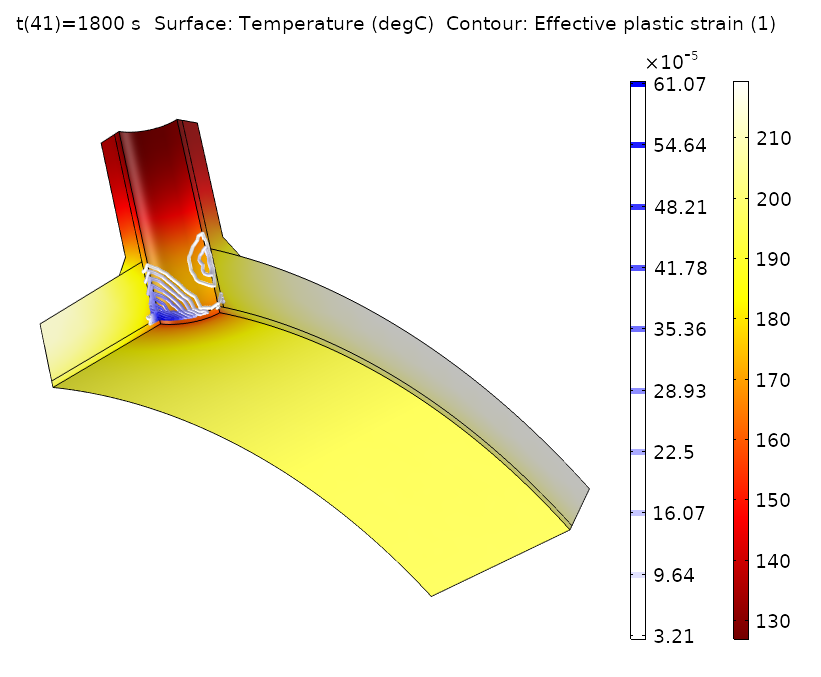
A pressure vessel is subjected to a rapid temperature change. The temperature gradients during the cooling cause plastic deformations in the stainless steel cladding, where the yield stress and hardening functions depend on the temperature. Instead of computing the time-dependent temperature field and the resulting plastic deformations simultaneously, the problem is split into three separate studies:

1. Initialization step to get the initial stress and temperature distribution due to the temperature and pressure conditions inside and outside of the vessel
2. Transient analysis of the temperature development due to cold water that suddenly flows into the vessel through pipes
3. A sequence of stationary study steps that uses the resulting transient temperature field to compute the development of the elastoplastic deformations

The sequence of studies described above is justified by two key assumptions:

• We can use the fact that the deformations do not affect the temperature field. (A side note: Physically there could be a very small such effect, but in order to capture it, the heat transfer between the fluid and the structure would have to be computed using a full fluid-structure analysis, rather than being prescribed using a convection condition.)
• The deformation can be regarded as instantaneous in relation to the time scale, which is why there is a stationary solution for the mechanical analysis at each point in time.

To set up this fairly complex sequence, nothing more is needed than to select the correct initial conditions from the previous study steps and define a time parameter t, which is used as a placeholder for the final parametric stationary study. The deformations are automatically computed using the values from the respective time point in the thermal study.

Temperature field and effective plastic strain in a pressure vessel after a massive temperature drop.

Modeling a Cross-Flow Heat Exchanger with a One-Way Coupling

Let’s try out the one-way coupling approach using a nonisothermal flow example, the Cross-Flow Heat Exchanger tutorial model. This type of heat exchanger is found in lab-on-a-chip devices in biotechnology and microreactors, such as for microsized fuel cells.

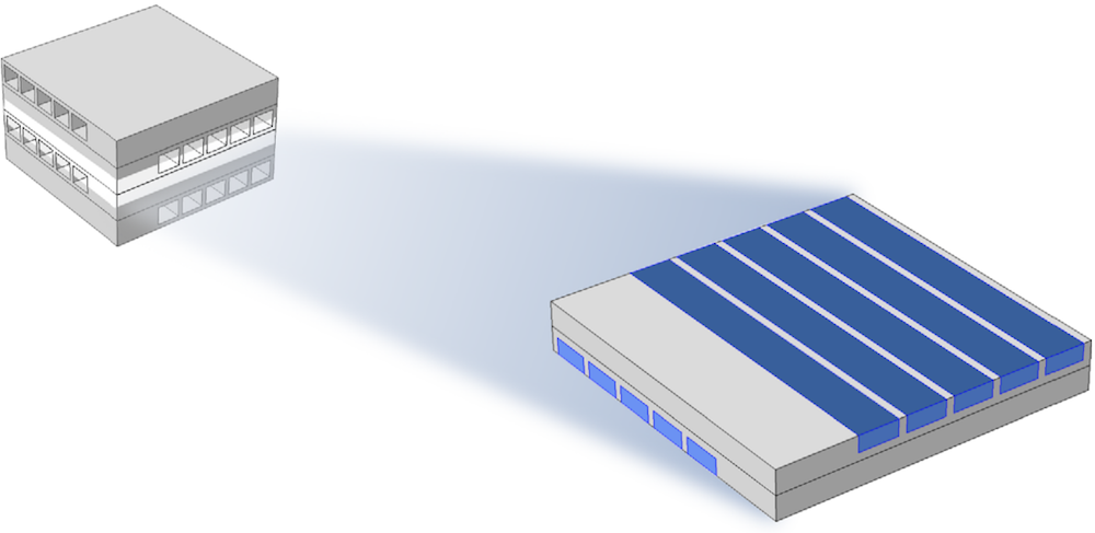
The modeled part of the microsized heat exchanger.

The modeled system consists of two sets of channels, one hot and one cold, arranged in a cross-flow pattern with five channels in each set, as shown in the figure above. The model is reduced due to the symmetry of the heat exchanger.

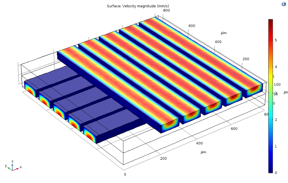
If we check the study nodes of the model, we find two stationary study steps. In the first study step, only laminar flow (spf) is selected for solving, while in the second study step, heat transfer (ht) is selected together with the multiphysics coupling nonisothermal flow (nitf1). The flow field is solved in the first study step and the result is automatically taken in the second step because of the applied coupling provided by the Nonisothermal Flow multiphysics node. This study setup, preset and available as of COMSOL Multiphysics version 5.3, is called Stationary, One-Way Coupled, NITF for stationary simulations and Time Dependent, One-Way Coupled, NITF for transient simulations.

Comparing the Results for the One-Way and Two-Way Couplings

We can compare the results of the one-way coupled approach with a two-way coupled version by adding a new study with a stationary, fully coupled study step. After computing both studies, it turns out that the results differ only slightly. The average heat transfer coefficient on the upper channel walls, probably the most interesting result of the model, becomes 3147.7 W/(m2K) for the two-way coupling and 3147,5 W/(m2K) for the one-way coupling. The difference of 0.2 is probably a lot smaller than the numerical error in the two computations. Further, the computation time is halved — from about 83 seconds for the two-way coupled problem to half a minute for the one-way coupled problem.

A comprehensive comparison of the two approaches can be found in the slideshow presentation available with the model documentation.

Temperature results of the one-way coupling (left) and two-way coupling (right) stationary solutions.

If the transient behavior of the model is of interest, other study combinations are possible. For example, we can add two time-dependent study steps, where the flow is solved first, followed by a transient heat transfer study step (Time Dependent, One-Way Coupled, NITF). We can also create a study sequence with a stationary flow and a transient heat transfer study if the flow conditions are not changed with time (except temperature). The table below gives an overview of the different study combinations and their respective computation times for a simulation time of 10 seconds.

The computation times of different study approaches on an Intel® Xeon® W-2135 @ 3.70 GHz machine.

As expected, cases where the transient heat transfer is one-way coupled with stationary flow fields are computed faster. The demonstration problem is obviously small with respect to the computational time, but the simplified approach discussed in this blog post becomes a more important option as a problem grows.

Want to learn more about how the COMSOL® software can fit your modeling needs? Click the button below to evaluate the software:

Further Reading

• Read these related blog posts:
  • Compressibility Options and Buoyancy Forces for Flow Simulations
  • Characterizing the Flow and Choosing the Right Interface

 
Intel and Intel Xeon are trademarks of Intel Corporation in the U.S. and/or other countries.