How to Use Maximum Likelihood for Parameter Estimation in COMSOL®

Parameter estimation rarely lends itself to eye-catching illustrations, but it often plays an important role for getting accurate material data and thus accurate simulation results. It involves minimizing the difference between measured experimental results and the corresponding data in the model. Sometimes, you may need to combine data from several experiments, which requires setting appropriate weights so that all experiments contribute information to the estimated material parameters. Maximum likelihood parameter estimation provides a way to choose the weights automatically based on objective criteria, so that the maximum amount of information is extracted from the experiments.

Avoiding Manual Tuning with the Method of Least Squares

The method of least squares is a special case of maximum likelihood parameter estimation that is a good starting point for basic parameter estimation, making it a popular approach. The COMSOL Multiphysics® software comes with built-in support for the least-squares method.

In this post, we will demonstrate how utilizing maximum likelihood parameter estimation can help avoid the need to manually tune weights for a given problem.

In this example, the relative error of the two parameters depends on the weights chosen for the two sets of measurements. Determining both parameters accurately thus requires that a good compromise is found between the two weights.

Probability and Statistics When Data Sampling

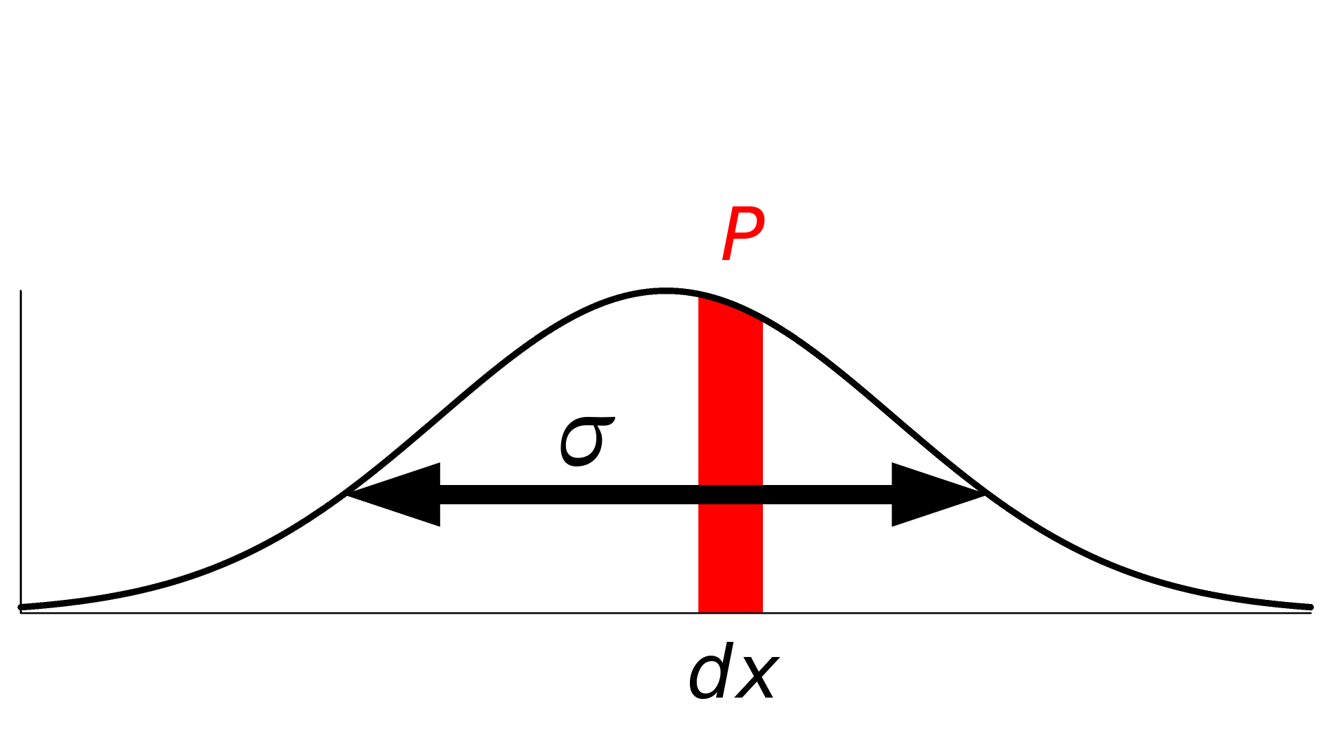
The probability P of sampling a data point in a certain range [a, b] for a probability density function f is given as the integral

In this context, we only consider an infinitesimal range dx around a measurement x, so the probability becomes

In this sense, there is a direct relationship between the probability density function and the probability given by dx. (dx can be omitted for notational convenience.)

The probability of sampling a certain value can be computed by integrating the probability density function.

Least-Squares Objectives and Maximum Likelihood Parameter Estimation

Different sources of discrepancies between the simulation and the experiment can be considered. In the following example, we will consider normally distributed uncertainties from the actual measurement, so the probability of measuring a value x^e becomes

where \sigma is the standard deviation of the measurement error and x is the mean value. For n measurements, we can compute the joint likelihood as the product

We can take the logarithm of the likelihood to avoid the products and any associated numerical difficulties. We then get a sum instead, which resembles a least-squares objective:

In a sense, we can say that \sigma plays the role of weight in a least-squares objective. Therefore, to maximize the likelihood, we need to minimize the right-hand side of the equation, and regardless of \sigma, the minimum will occur when the sum of the squared deviations takes the minimum value. If there are different sets of measurements with different \sigma, we cannot draw the same conclusion. Let’s investigate such an example.

Maximum Likelihood for a Tensile Test

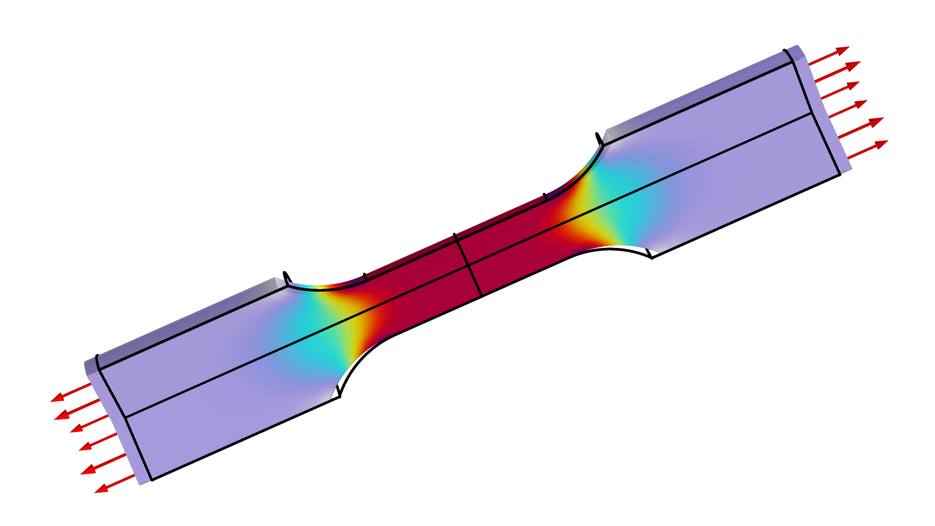
It is common to estimate Poisson’s ratio of materials with a compression test, but for the sake of demonstration, we will consider an example where Poisson’s ratio as well as Young’s modulus is estimated using a tensile test. We will do this by measuring the tensile force and the radial shrinking in the test specimen illustrated in the figure below.

The figure shows the stress for a tensile test. The force and the center radial displacement are measured as functions of the stretching.

There is a difference of around 10 orders of magnitude between the force and displacement measurement data (for SI units), so with a regular least-squares approach, we would need to tune the weights of the least-squares objective to get accurate results for both material parameters. However, we can compute the optimal weights with maximum likelihood automatically by using the standard deviation of the two measurements errors \sigma_F and \sigma_r as controls; i.e.,

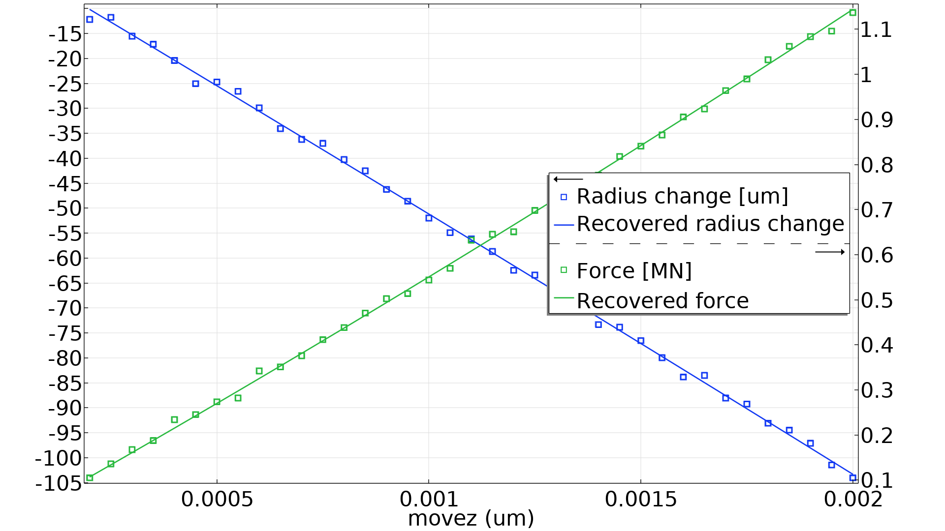
The built-in support for least-squares objectives in COMSOL Multiphysics makes it quite straightforward to define custom objectives in order to solve maximum likelihood parameter estimation problems. The Parameter Estimation Using Maximum Likelihood model, available in the Application Gallery, generates synthetic data by adding normally distributed noise. The model then recovers the material parameters and the standard deviations based on this data. The resulting force and radial displacement are shown in the figure below.

The noisy data and optimized model behavior are plotted as functions of the stretching. There are 37 data points for each of the two measurements.

The model is able to recover the material parameters to an accuracy of 0.1–0.5% and the standard deviations to around 6%, but the accuracy is expected to increase with the number of measurements.

In this post, we have focused on the case of normally distributed noise with a fixed standard deviation, but the framework of maximum likelihood parameter estimation can be extended to fit the realities of specific experiments so that information is extracted in an optimal and consistent way.

Try It Yourself

Try the Parameter Estimation Using Maximum Likelihood model yourself by clicking the button below, which will take you to the Application Gallery entry:

Further Resources

Explore more examples of parameter estimation with these models:

• General Parameter Estimation
• Impedance Tube Parameter Estimation with Data Generation
• Aquifer Characterization

Check out these resources to learn more about parameter estimation:

• Blog post: How to Use the Parameter Estimation Study Step for Inverse Modeling
• Video: Performing Parameter Estimation in COMSOL Multiphysics®