How to Use the v2-f Turbulence Model in the CFD Module

Accurately modeling turbulent flow is always a challenge with turbulence models, since they inherently involve simplifications. In addition, accurate models tend to add equations that don’t help the convergence of the already highly nonlinear models. To solve this problem, version 5.3 of the COMSOL Multiphysics® software introduces the v2-f turbulence model. It combines the accuracy obtained with models that describe the anisotropy of the turbulent boundary layers with the robustness of two-equation turbulence models.

Modeling CFD with the v2-f Turbulence Model

The transport of momentum normal to the boundary in turbulent boundary layers is strongly damped by the presence of the solid wall. Also, the normal component of the turbulence intensity is more strongly suppressed by the proximity to the solid wall than the in-plane components. This means that mass and heat transfer in the normal direction to the wall are also partly blocked. Traditionally, this blocking effect has been dealt with by introducing damping functions for the normal component of the turbulent viscosity in wall-resolved turbulence models.

Using direct numerical simulations, Durbin confirmed that the near-wall damping of the eddy viscosity is caused by the suppression of the turbulence intensity’s normal component according to the following relation:

(1)

where C_μ denotes a model constant, \[\overline {{v^2}} \] is the variance of the normal component of the turbulent velocity, and T represents the turbulence time scale.

The effect of the wall on the damping of the turbulence intensity is depicted in the figure below. The distance from the surface of a bubble or platelet-shaped object from their centers represents an average of the turbulence intensity at the centerpoint of the bubble or platelet shape.

Close to the walls, the fluctuations of the velocity are much larger in the x direction and y direction in comparison with the z direction. The velocity fluctuations are anisotropic and the surface takes the shape of a platelet. Further away from the wall, the fluctuations are of the same magnitude in all three dimensions: x, y, and z. The velocity fluctuations are isotropic and the surface takes the shape of a spherical bubble. The relative size of the bubbles and platelet shapes represents the relative size of the fluctuating eddies in the different directions.

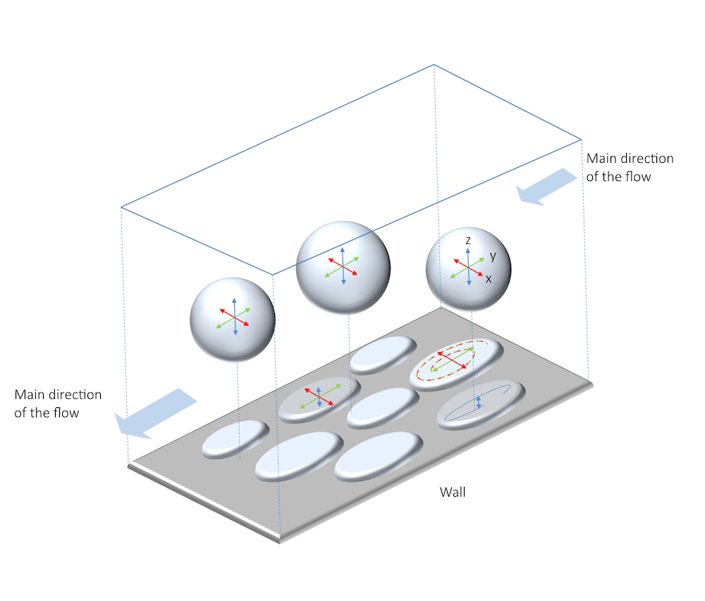
A representation of the average velocity fluctuations as imaginary bubbles or platelet shapes. The distance from the surface to the center of the bubbles or platelets represents the average magnitude of the turbulence intensity.

The v2-f turbulence model describes the anisotropy of the turbulence intensity in the turbulent boundary layer using two new equations, in addition to the two equations for turbulence kinetic energy and dissipation rate. The implementation used in the CFD Module, an add-on product to COMSOL Multiphysics, is based upon the formulation by F. Billard, J. Uribe, and D. Laurence from their 2008 paper.

The v2-f Turbulence Model Equations

To accurately describe the transport of turbulence energy and the redistribution of the turbulence energy in different directions, the v2-f model introduces two new equations. The first equation describes the transport of turbulence normal to the wall using a variable that is equal to \[{{\overline {{v^2}} } \mathord{\left/ {\vphantom {{\overline {{v^2}} } k}} \right. \kern-\nulldelimiterspace} k}\] (usually denoted φ or ς in scientific literature). In this equation, \[\overline {{v^2}} \] denotes the variance of the normal component of the turbulent velocity and k denotes the turbulence kinetic energy.

The second equation is an elliptic partial differential equation for the blending coefficient (usually denoted α in scientific literature). The elliptic blending equation accounts for nonlocal effects such as the wall-induced damping of the redistribution of turbulence kinetic energy between the normal and parallel directions. Due to the name of the independent variables, this model is often referred to as the φ-α version of the v2-f turbulence model. The model is equally as robust as standard isotropic turbulence models and as accurate as the original, less robust formulation of the v2-f model.

Example 1: Periodic Hill Benchmark

The implementation in the CFD Module has been verified using a few benchmark cases, including the periodic hill benchmark. In this model, a flow is forced over two parallel hills where the velocity field is periodic on the two vertical inlet and outlet boundaries (shown in the figure below). This means that while there is a pressure drop from the inlet to the outlet boundary, their velocity fields are identical.

In the figure below, the flow is from left to right. We can see that there is a detachment of the flow with a formation of a recirculation zone behind the hills in the direction of the flow. The size of the recirculation zone and the distance from the inlet to the reattachment of the flow is inherently difficult to predict using RANS turbulence models. The results obtained with the implementation of the CFD Module are in excellent agreement with the results reported in scientific literature.

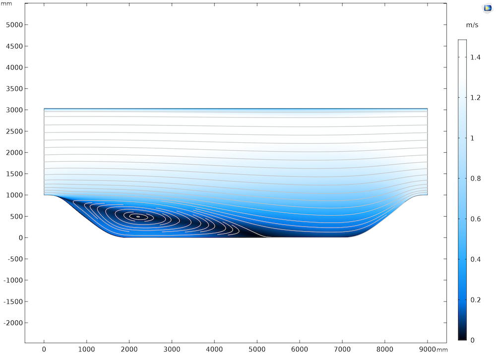
Flow over two hills where the velocity profiles at the vertical boundaries above the two hilltops are identical for the inlet and outlet boundaries. The flow is from left to right.

Example 2: Flow in a Hydrocyclone

Another interesting problem is the flow in a hydrocyclone with two tangential inlets. The two outlets are at the top and bottom. The stream from the bottom usually contains the undesired particles, thus it is called the reject stream. The outlet stream at the top is referred to as the accept stream. The difficulty is to capture the semifree vortex, which is unattainable for standard two-equation models.

For more information about hydrocyclone simulations, see this research paper.

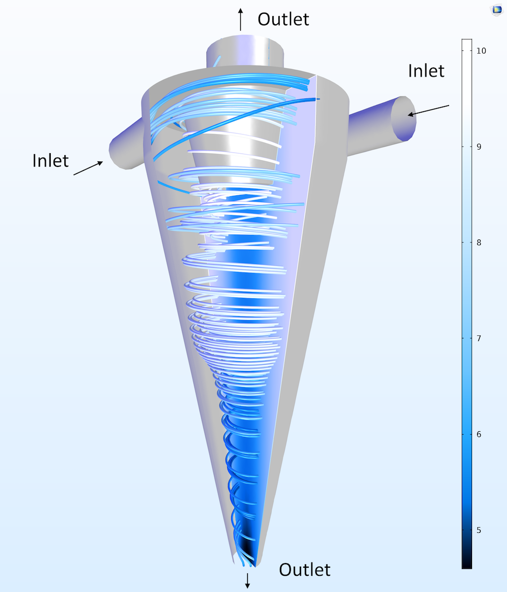
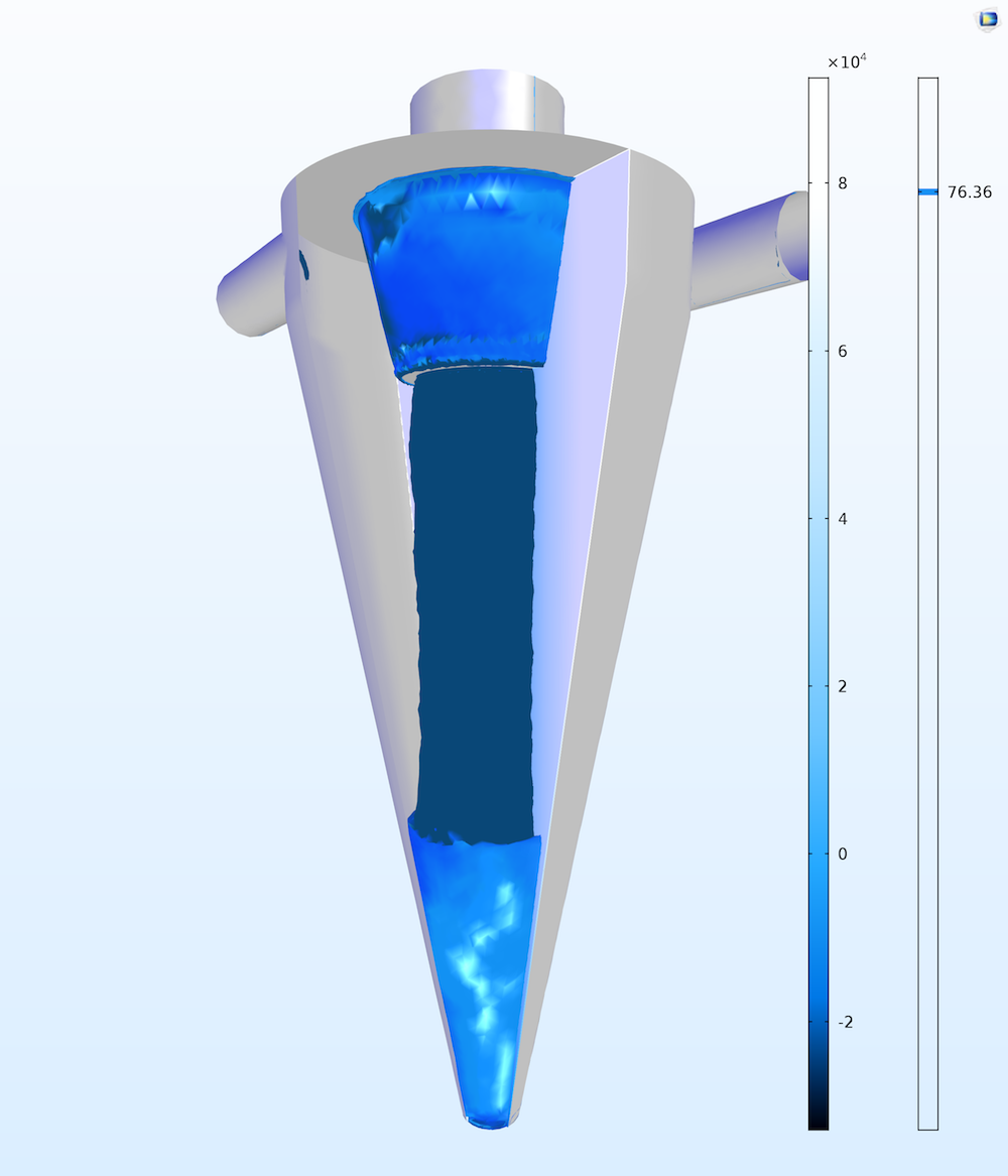
Left: Velocity field (streamlines) and pressure field (cross-section plot) in a hydrocyclone. Right: Isosurface of the absolute value of the vorticity in the cyclone and pressure cross section. The simulation captures the free vortex in the center of the cyclone.

The figure below shows the azimuthal component of the velocity just below the top outlet. The profile with a maximum at a radial position just outside of the outlet pipe is in good agreement with the results reported in scientific literature. In addition, the decrease of the azimuthal velocity away from the maximum outward along the radius is in good agreement with the literature.

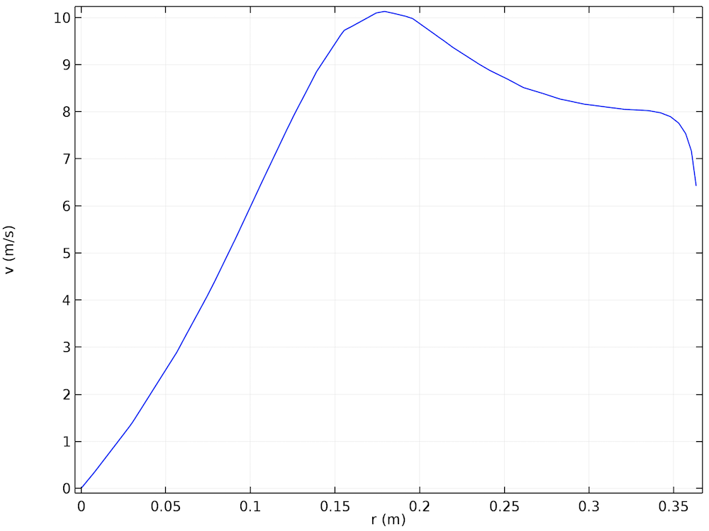
Azimuthal component of the velocity as a function of the radius in the cyclone just below its horizontal top outlet.

To summarize, the new v2-f turbulence model widens the applicability of the CFD Module to include cases that require anisotropic turbulence modeling. This model gives an accuracy that is not possible to obtain with two-equation models, yet it is as robust as standard two-equation models.

Additional CFD Resources

• Try it yourself: Get the hydrocyclone tutorial model
• Find out more about the updates to the CFD Module on the Release Highlights page