Introducing Nonlinear Elastic Materials

Nonlinear elastic materials present nonlinear stress-strain relationships even at infinitesimal strains — as opposed to hyperelastic materials, where stress-strain curves become significantly nonlinear at moderate to large strains. Important materials of this class are Ramberg-Osgood for modeling metals and other ductile materials and nonlinear soils models, such as the Duncan-Chang model.

Power Law

The nonlinear stress-strain behavior in solids was already described 100 years ago by Paul Ludwik in his Elemente der Technologischen Mechanik. In that treatise, Ludwik described the nonlinear relation between shear stress \tau and shear strain \gamma observed in torsion tests with what is nowadays called Ludwik’s Law:

(1)

For n=1, the stress-strain curve is linear; for n=2, the curve is a parabola; and for n=\infty, the curve represents a perfectly plastic material. Ludwik just described the behavior (Fließkurve) of what we now call a pseudoplastic material.

In version 5.0 of the COMSOL Multiphysics simulation software, beside Ludwik’s power-law, the Nonlinear Structural Materials Module includes different material models within the family of nonlinear elasticity:

• Ramberg-Osgood
• Power Law
• Uniaxial Data
• Bilinear Elastic
• User Defined

In the Geomechanics Module, we have now included material models intended to represent nonlinear deformations in soils:

• Hyperbolic Law
• Hardin-Drnevich
• Duncan-Chang
• Duncan-Selig

An Example with Uniaxial Data

The main difference between a nonlinear elastic material and an elastoplastic material (either in metal or soil plasticity) is the reversibility of the deformations. While a nonlinear elastic solid would return to its original shape after a load-unload cycle, an elastoplastic solid would suffer from permanent deformations, and the stress-strain curve would present hysteretic behavior and ratcheting.

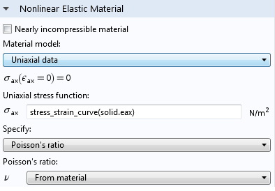
Let’s open the Elastoplastic Analysis of a Plate with a Center Hole model, available in the Nonlinear Structural Materials Model Library as elastoplastic_plate, and modify it to solve for one load-unload cycle. Let’s also add one of the new material models included in version 5.0, the Uniaxial data model, and use the stress_strain_curve already defined in the model.

Here’s a screenshot of what those selections look like:

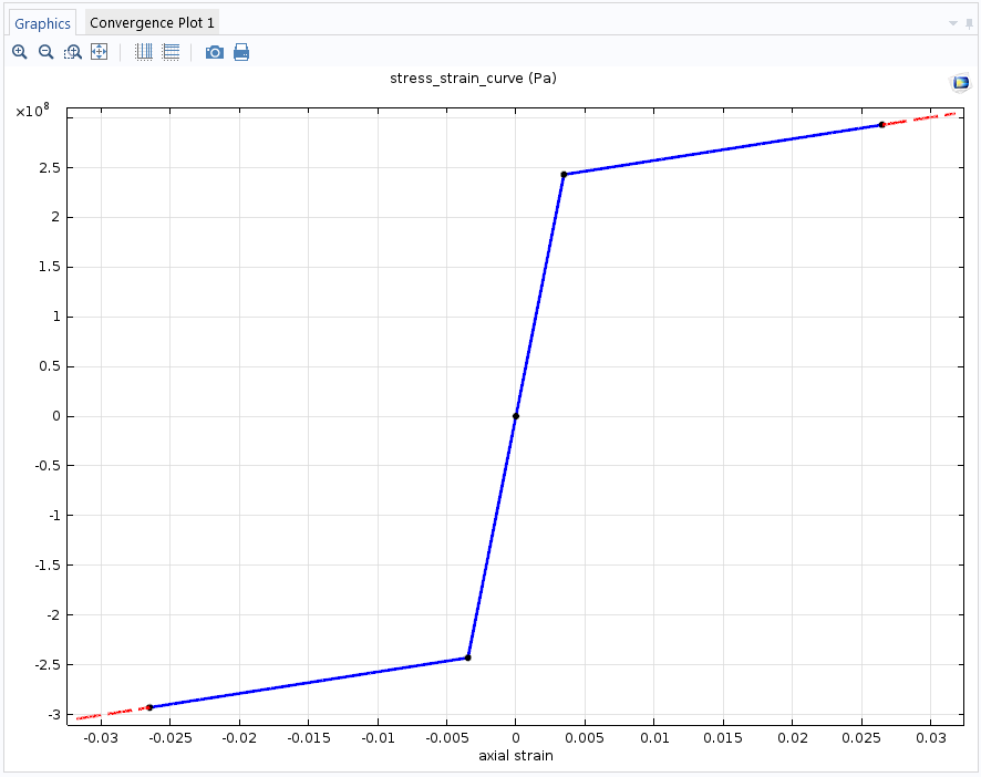
In our example, the stress_strain_curve represents the bilinear response of the axial stress as a function of axial strain, which can be recovered from Ludwik’s law when n=1.

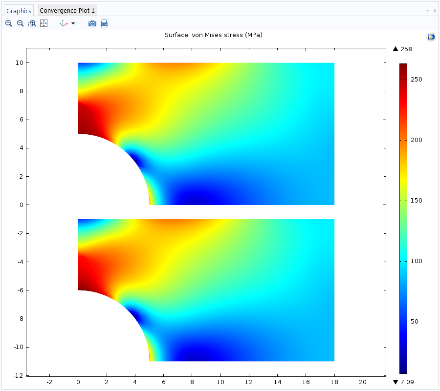
We can compare the stress distribution after laterally loading the plate to a maximum value. The results are pretty much the same, but the main difference is observed after a full load-unload cycle.

Top: Elastoplastic material. Bottom: Uniaxial data model.

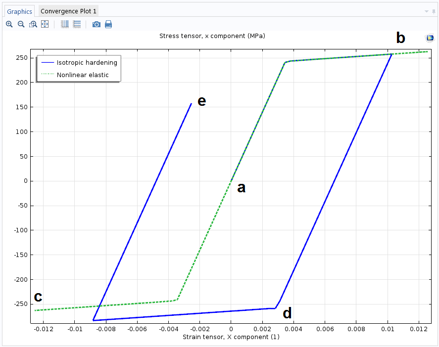
Let’s pick the point where we observed the highest stress and plot the x-direction stress component versus the corresponding strain. The green curve shows a nonlinear, yet elastic, relation between stress and strain (the stress path goes from a\rightarrow b \rightarrow a \rightarrow c \rightarrow a). The blue curve portraits a hysteresis loop observed in elastoplastic materials with isotropic hardening (the stress path goes from a\rightarrow b \rightarrow d \rightarrow e ).

With the Uniaxial data model, you can also define your own stress-strain curve obtained from experimental data, even if it is not symmetric in both tension and compression.

Further Reading

• P. Ludwik. Elemente der Technologischen Mechanik
• “Hypoelasticity“, Chapter 3.3 of Applied Mechanics of Solids
• Download the Elastoplastic Analysis of a Plate with a Center Hole model