When modeling plasmas, various options exist for choosing an ion temperature. Your choice, however, may strongly influence your model’s results. Let’s discuss the theoretical reason behind this phenomenon and study an example involving an inductively coupled plasma (ICP) to illustrate the influence the different ion temperature options have on your model’s results.
Choosing an Ion Temperature
Non-equilibrium cold plasmas are characterized by an electron temperature that is much higher than the gas temperature. During plasma modeling, the ion temperature is often set to equal the gas temperature. This is an acceptable approximation, as long as the ions undergo sufficient collisions with neutral gas molecules and then thermalize with the background gas. This is especially true in inductively coupled plasmas (ICP), where the pressure is low and the ions’ mean free path length comes closer to the plasma reactor’s length scale. Moreover, the number of collisions are low, therefore, the ion temperature is somewhere in between the gas and electron temperatures.
While COMSOL Multiphysics does not solve for the ion temperature, there are some options available for you to do so.
You can choose to set the ion temperature to equal the gas temperature or use a user-defined value or expression. Moreover, you can also elect to define a correlation between the electric field and the ion mobility and employ an Einstein relation to calculate it, using the Local Field Approximation (LFA) — available in the COMSOL software.
As mentioned, your choice in ion temperature (especially for low-pressure plasmas) could significantly impact your model’s results. Below, you will find a theoretical reason that helps explains this phenomenon.
Theoretical Background
For the heavy species transport (and ion transport), a continuity equation with a drift diffusion approximation is solved for each species. The variation of the mass fraction ,w_k, for species k depends on a flux, \mathbf{j}_k, and a reaction term, R_k. In this case, convection and thermal diffusion are neglected for simplicity:
To compute the flux, \mathbf j_k, a mixture averaged diffusion coefficient, D_{k,m}, and the ion mobility, \mu_{k,m}, are required:
Based on the kinetic theory of gases, binary diffusion coefficients, D_{kj}, are calculated to get the mixture averaged diffusion coefficient, D_{k,m}. You may have already noticed that Lenard-Jones parameters, \sigma and \epsilon / k_B, have to be specified for each plasma species:
The ion mobility is then calculated, using an Einstein relation according to:
At the reactor walls, the ion flux, \mathbf j_k, to the wall, is computed according to:
The ion temperature is needed to compute the ion mobility and flux to the reactor walls, so the choice in ion temperature especially affects the ions’ transport properties within the plasma model. If the migration part of the flux is large, in comparison to the diffusion part, then the choice in ion temperature particularly grows in importance. This is notably true in cases at very low pressures or at high electric field strengths.
Using the Local Field Approximation (LFA)
To reiterate, you can also compute the ion temperature with the help of the LFA, available in COMSOL Multiphysics.
The LFA assumes that the local velocity distribution of the particles is balanced with the local electric field. Therefore, quantities, like ion temperature or ion mobility, can be expressed in terms of (reduced) electric field. The LFA requires that local changes in the electric field are small in comparison to the mean free path length. However, this is not always true in the boundary layer, particularly.
The following expression, for the reduced electron mobility as a function of the reduced field, is used in a subsequent ICP example, below.
In the equation above, the reduced electric field,E/n, is given in Townsends (Td).
Inductively Coupled Plasma Example
To demonstrate the impact your ion temperature choice has on an ICP model, let’s take a look at an example.
An inductively coupled plasma reactor (similar to the GEC ICP Reactor, Argon Chemistry model) was modeled three times with varying ion temperatures. Because ICPs work at particularly low pressures, the ion temperature choice has to be considered carefully.
The ion temperature was:
- set to 300 K, which corresponds to the gas temperature, in Model 1.
- set to 0.1 eV (1160 K), which corresponds to a typical literature value, in Model 2.
- set to D_{k,m} / \mu_{k,m}, while \mu_{k,m} was computed with the LFA , in Model 3.
The other model parameters were as follows:
| Model Parameters | |
|---|---|
| Gas Temperature | 300 K |
| Coil Power | 500 W |
| Pressure | 0.02 torr |
| Electron Mobility | 4E24 (1/(m*V*s)) |
The mean ion temperature from Model 3, which was computed from D_{k,m} / \mu_{k,m}, amounts to 0.22 eV –, or 2515 K.
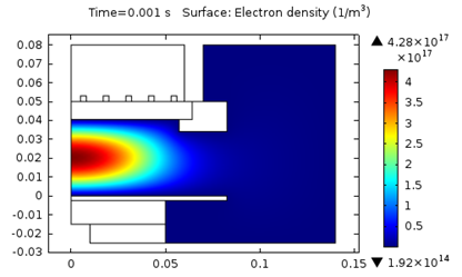
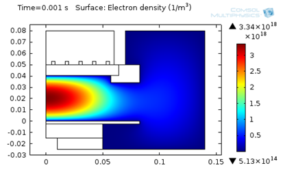
The following figures represent the electron density for all three models after 0.001 seconds.

Model 1: Electron density (T_ion = 300 K).

Model 2: Electron density (T_ion = 0.1 eV).

Model 3: Electron density (T_ion from LFA).
As seen above, using a higher ion temperature value significantly increases the electron density.
The modeling results are also compared in the table below. The maximum electron density, maximum electron temperature, and the absorbed power are displayed.
| Max. Electron Density [1/m³] | Max. Electron Temperature [eV] | Resistive Losses [W] | |
|---|---|---|---|
| 1. T_i = 300 \text K | 4.3E17 | 4.1 | 387 |
| 2. T_i = 0.1 \text {eV} | 2.6E18 | 2.8 | 407 |
| 3. Local Field Approximation | 3.3E18 | 2.3 | 41 |
Based on the table, we can deduce that increasing the ion temperature not only leads to a significant increase in electron density, but also the absorbed power. Additionally, the electron temperature noticeably decreases.
The example above illustrates the impact the choice in ion temperature has on the modeling results of an ICP. A comparison of the results with literature values is essential in judging which assumptions give the best outcomes.


Comments (1)
Pouyanesh Co.
October 14, 2020Hello
I can not found the example with local field approximation. Can you help me?