Modeling a Coil Heat Exchanger

Coil heat exchangers are simple and easy to manufacture. Here, we consider an axially wound coil of copper carrying hot water that heats air inside of a circular duct. Since the geometry is almost invariant about the centerline, the model is solved in the 2D axisymmetric plane. Additional expressions are added to compute the temperature drop between turns of the coil, which greatly simplifies the modeling.

A Coil Heat Exchanger Model

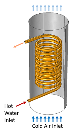
The coil heat exchanger we’ll consider is shown in the figure below.

A copper coil carries hot water through a duct carrying cold air.

Copper tubing is helically wound so that it can be inserted along the axis of a circular air duct. Cold air is moving through the duct, and hot water is pumped through the tubing. The air flow pattern and the temperature of the air and copper pipes will be computed using the Conjugate Heat Transfer interface. Since the geometry is almost axisymmetric, we can simplify our modeling by assuming that the geometry and the air flow are entirely axisymmetric. Thus, we can use the 2D axisymmetric Conjugate Heat Transfer interface. Since the airspeed is high, a turbulent flow model is used; in this case, it is the k-epsilon model.

We can assume that the water flowing inside of the pipe is a fully developed flow. We can also assume that the temperature variation of the water is small enough that the density does not change, hence the average velocity will be constant. Therefore, we do not need to model the flow of the water at all and can instead model the heat transfer between the fluid and the pipe walls via a forced convective heat transfer correlation.

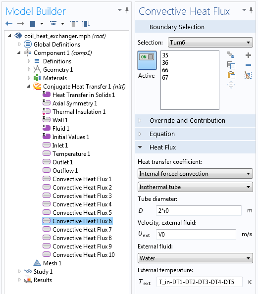
The Convective Heat Flux boundary condition uses a Nusselt number correlation for forced internal convection to compute the heat transfer between the water and copper tubing. This boundary condition is applied at all inside boundaries of the copper piping. As inputs, it takes the pipe dimensions, fluid type, fluid velocity, and fluid temperature. With the exception of the fluid temperature, all of these quantities remain constant between the turns of the tubing.

Modeling the Temperature Drop Between Turns

As the hot water is being pumped through the copper coils, it cools down. However, since the model is axisymmetric, each turn of the coil is independent of the others, unless we explicitly pass information between them. That is, we must apply a separate Convective Heat Flux boundary condition at the inside boundaries of each coil turn.

This raises the question: How do we compute the temperature drop between each turn and incorporate this information into our model?

Consider the water passing through one turn of the copper coil. The heat lost by the water equals the heat transfer into the copper pipes. Under the assumption of constant material properties, and neglecting viscous losses, the temperature drop of the water passing through one turn of the pipe is:

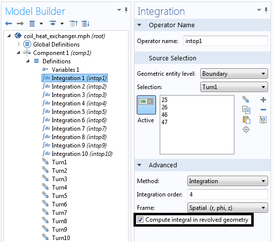
where \dot m is the mass flow rate, C_p is the specific heat of water, and Q is the total heat lost by the water, which is equal to the integral of the heat flux into the copper, integrated over the inside boundaries of the coil. This integral can be evaluated via the Integration Component Coupling, defined over the inside coil boundaries.

The Integration Component Coupling defined over a boundary. Note: The integral is computed in the revolved geometry.

Using these coupling operators, we can define a set of user-defined variables for the temperature drop:

DT1 = intop1(-nitf.nteflux/mdot0/Cp0)

This evaluates the temperature drop along the first turn of the pipe. We can define a different temperature drop variable for each turn of the pipe and use them sequentially for each turn.

The water temperature in the sixth turn considers the temperature drop in the first five turns.

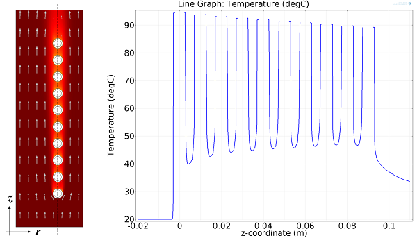
Flow field and temperature plot (left) and the temperature along a line through the center of the coils (right).

Since this is a 2D axisymmetric model, it will solve very quickly. We can examine the temperature and the flow fields and plot the temperature drop along a line down the center of the coils. We can observe that the water cools down between each turn of the coil, and the air heats up.

This can be considered a parallel-flow heat exchanger, since the hot and cold fluids flow in the same overall direction. If we wanted to change this model to the counter-flow configuration, we could simply switch the air inlet and outlet conditions so that the fluids travel in opposite directions.

What other kinds of heat exchanger configurations do you think this technique can be applied to?