
Guest blogger Björn Fallqvist from Lightness by Design discusses different considerations and approaches for analyzing thermomechanical fatigue.
In this blog post, we investigate the relevant material models in the COMSOL Multiphysics® software for analyzing thermomechanical fatigue. Experimental data from thermomechanical fatigue tests are used, along with material parameters from the referenced literature. Subsequently, a pressure vessel assumed to be operating at elevated temperatures is analyzed, and a nonlinear continuous fatigue damage model is used to assess the fatigue life.
Why Analyze Thermomechanical Fatigue?
In many applications, traditional isothermal fatigue analysis is not sufficient, as the components operate at, or are cycled between, elevated temperatures, where the material behavior differs significantly from room temperature. Typical examples of such applications are turbines and power plant components.
Traditional fatigue analysis, especially high-cycle fatigue (HCF), does not directly account for effects due to high temperature. In the HCF region, the loads are low and effects such as creep are assumed to be negligible. Sometimes, a reduction of the S-N curve is made to account for reduced fatigue strength at increased temperature. However, this does not take into account the effect of cycling the temperature and load simultaneously, known as thermomechanical fatigue. The effect of this variation in temperature is especially important in the low-cycle fatigue (LCF) region, where multiple aspects need to be taken into account — primarily the variation of material properties for elastoplasticity and creep.
One way to assess the fatigue capability at elevated temperatures is to use the stabilized (often midlife) stress-strain curve of a specimen at several temperatures to obtain a stress or strain amplitude and determine the hardening parameters governing the nonlinear stress-strain curve. One could then, in theory, conduct experiments with a particular set of combinations of applied load and temperature and attempt to estimate the fatigue life from experimental results. Thermomechanical fatigue testing, however, takes a relatively long time and is costly. A more convenient way of assessing the fatigue capability at elevated temperature is to use an analytic expression for the relation between stress levels and cycles to failure and correct it for temperature.
Thermomechanical Fatigue Testing
In thermomechanical fatigue testing, a specimen is typically subjected to a cyclic strain and cyclic temperature simultaneously. This can be either in-phase (IP) or out-of-phase (OOP). For the former, the maximum tensile load occurs at the same time as the maximum temperature, and in the latter case, the maximum tensile load occurs at the minimum temperature.
For comparison with experimental results in this blog post, we refer to Ref. 1, in which the thermomechanical fatigue of a P91 (a common power plant steel) was investigated. Stress-strain curves were obtained, and material model parameters were taken from Ref. 2. It is worth noting that for the referenced work, a unified model (i.e., the viscoplastic strains are composed of both the plastic and creep components) is used. This will only affect the values of the creep part of the model, however.
Material Models for Thermomechanical Fatigue Analysis
The material model parameters as a function of temperature (Ref. 2) are as specified below:
| Temp [°C] | E [MPa] | k [MPa] | Q [MPa] | b [-] | a1 [MPa] | C1 [-] | a2 [MPa] | C2 [-] | Z [MPa s1/n] | n [-] |
|---|---|---|---|---|---|---|---|---|---|---|
| 400 | 187,537.0 | 96 | -55.0 | 0.45 | 150.0 | 2350.0 | 120.0 | 405.0 | 2000 | 2.25 |
| 500 | 181,321.6 | 90 | -60.0 | 0.6 | 98.5 | 2191.6 | 104.7 | 460.7 | 1875 | 2.55 |
| 600 | 139,395.2 | 85 | -75.4 | 1.0 | 52.0 | 2055.0 | 463.0 | 463.0 | 1750 | 2.7 |
Table 1. Material parameters from reference.
The parameters a and C are related to the nonlinear kinematic hardening model, E is the elastic modulus, k is the initial yield stress, Q and b are isotropic hardening parameters, and Z and n are material parameters for the viscoplastic flow rate.
These will be elucidated upon in the following sections. Taken together, these parameters determine the translation and expansion/contraction of the yield surface in stress space. All parameter values in the model are interpolated between temperatures. The implementation of this will be shown in subsequent sections.
Viscoplasticity
Rate-dependent effects are taken into account by using the viscoplastic Chaboche formulation for the rate of the viscoplastic strain tensor \dot{\epsilon}_{vp} according to Ref. 5.
where A is a rate factor (set equal to 1/s), F is the yield function), nD is the tensorial direction of the stress deviator, n is a material parameter, and \sigma_{ref} is a reference stress value.
By inspection, the COMSOL Multiphysics parameters σref and n are equal to Z and n in Table 1, respectively. The yield function F is defined as
Here, R is the increase in yield surface, k the initial yield stress, and \sigma_b the backstress tensor due to kinematic hardening.
The function φ is chosen to be the von Mises equivalent stress.
Isotropic Hardening
The isotropic hardening law (Voce) for the yield surface size σy is defined as
where σsat is a saturation stress for the yield surface size at large plastic strains, β is a material parameter, and \epsilon_{vp,e} is the equivalent viscoplastic strain.
With this formulation, depending on the saturation stress value, the yield surface may either expand or contract with increasing plastic strain. The COMSOL Multiphysics parameters σsat and β correspond to Q and b in Table 1, respectively.
Kinematic Hardening
The chosen nonlinear kinematic hardening law is Chaboche hardening, where the backstress tensor consists of j number of superimposed branches of Armstrong–Frederick nonlinear hardening terms:
The first term, with an initial kinematic hardening modulus, is ignored in our analyses. By comparison to the formulation used in Ref. 1–2, the hardening parameters C and γ for the two branches in COMSOL Multiphysics are Ca and C, respectively.
Creep
As mentioned previously, in the referenced articles, the authors used a unified viscoplastic model, and the viscous stress is defined directly. In COMSOL Multiphysics, we use the Norton creep model for the rate of creep strain:
Here, Ac is a rate factor, σeff is the equivalent stress, σref is a reference stress value (set to 1 MPa), and nc is a material parameter. The values of these parameters were taken from Ref. 6.
Summary of Material Parameters for Use in COMSOL Multiphysics®
The material parameters used in the analyses are summarized below. Note that the parameter names have, in most cases, been changed to reflect the labels in COMSOL Multiphysics. Also, the definition of the constants C differs from that used in the referenced article, hence they take on a different value.
| Temp [°C] | E [MPa] | \sigma_{ys0} [MPa] | \sigma_{sat} [MPa] | β [-] | C_1 [MPa] | \gamma_1 [-] | C_2 [MPa] | \gamma_2 [-] | \sigma_{ref,vp} [MPa s1/n] | n [-] |
|---|---|---|---|---|---|---|---|---|---|---|
| 400 | 187,537.0 | 96 | -55.0 | 0.45 | 352,500 | 2350.0 | 810,000 | 405.0 | 2000 | 2.25 |
| 500 | 181,321.6 | 90 | -60.0 | 0.6 | 215,870 | 2191.6 | 863,810 | 460.7 | 1875 | 2.55 |
| 600 | 139,395.2 | 85 | -75.4 | 1.0 | 106,860 | 2055.0 | 810,250 | 463.0 | 1750 | 2.7 |
Table 2. Material parameters for use in COMSOL Multiphysics.
The creep parameters A_c=2.4623 \cdot 10^{-21}/h, \sigma_{ref,cr}=1 MPa, and n_c=7.538 were the same for all temperatures, as was the Poisson’s ratio of 0.3 and the coefficient of thermal expansion \alpha=14.5 \cdot 10^{-6}/^{\circ}C. Note that the creep parameters were measured at 873 K, although a temperature dependence can also be included in COMSOL Multiphysics.
Nonlinear Continuous Damage Fatigue Model
Background
The fatigue model we will use in the fatigue analysis is the nonlinear continuous fatigue damage model proposed by Chaboche (Ref. 3). This model is attractive thanks to its ease of use and its validity for both low- and high-cycle fatigue (for steels). Briefly, it is based on a rate damage equation of the form
The rate of the damage variable D with respect to cycles N depends on maximum stress \sigma_M, mean stress \bar\sigma, and current damage. With a particular choice for the function f, one ends up with (derivation omitted here) a relation for the number of cycles to failure, NF:
where a and \beta_{fat} are material parameters, \sigma_u is the ultimate tensile strength, and \sigma_l is the fatigue limit for the mean stress \bar\sigma according to
Here, b_{fat} is a material parameter.
Finally, M\bar{(\sigma)} is defined as
with M_0 as a material parameter.
In thermomechanical fatigue, where the temperature T varies, an effective temperature (T*) can be computed during a cycle according to
Essentially, the effective temperature T* is taken to be that for which the same number of cycles NF is computed, as the average number of cycles over a time span \Delta t between extreme temperatures.
Fatigue Data and Assumptions
At room temperature, the ultimate tensile strength of P91 steel is 600 MPa (Ref. 7), and the fatigue limit is approximately 420 MPa, taken from Ref. 6, along with the number of cycles to failure at varying stress levels. These can be used to determine a least-squares fit for the S-N curve as defined by the Chaboche fatigue model, Figure 1. Here, the load ratio R (R=\frac{\sigma_{min}}{\sigma_{max}}, ratio of minimum to maximum stress) is R = -1; i.e., \bar\sigma=0. For the parameter determination, M\bar{(\sigma)}=M_0 and \sigma_l(\bar\sigma)=\sigma_{l0}.
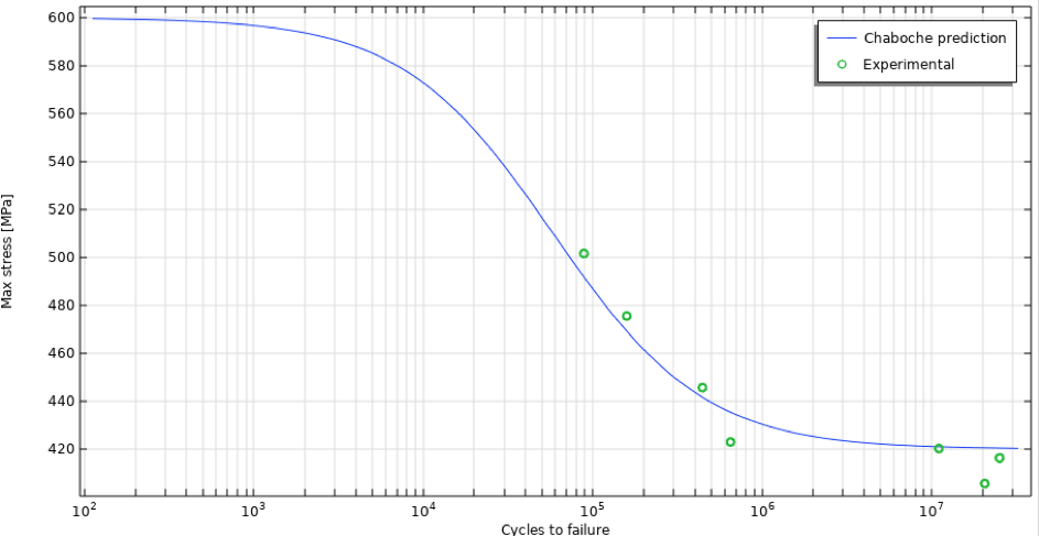
Figure 1. S-N curve as defined by the Chaboche fatigue model.
The resulting parameters are a = 9 \cdot 10^{-6}, \beta_{fat}=0.287, and M_0=54.3 MPa.
Ideally, more points in the intermediate region are needed to fully define the curve, but for a method demonstration, this will suffice. Since accounting for thermal effects is crucial, the S-N curve must be scaled. There are several ways to do this; the most proper would be to utilize curves at different temperatures, obtain material parameters for each temperature, and interpolate these. However, lacking such data, it is convenient to scale the ultimate tensile strength and fatigue limit according to reduction factors defined by Figure 3.24 in Ref. 1. The resulting S-N curves are shown in Figure 2. Note that these are all for R = -1.
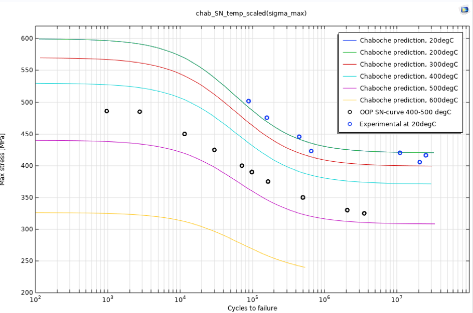
Figure 2. Chaboche S-N curves with temperature reduction.
The implementation of scaling these curves for temperature will be shown in the subsequent section. The computed cycles to failure for a selected number of stress levels, assuming an out-of-phase temperature cycling between 400°C and 500°C, defined by the setup in Ref. 2, is also included.
When it is necessary to account for mean stress effects, the parameter b_{fat} is needed. A Goodman reduction of the fatigue limit with respect to mean stress is used when necessary; i.e., when \bar\sigma=\sigma_u, \sigma_l=0. This yields b_{fat}=0.0041/MPa.
Computational Models
Background: Experimental Comparison
Experimental thermomechanical fatigue testing (isothermal and out-of-phase) was performed in Ref. 2. Uniaxial tensile tests were conducted at elevated temperatures, both under isothermal and anisothermal conditions. To demonstrate the process of defining the steps necessary for a thermomechanical fatigue analysis, the experimental setup and testing procedure are replicated in COMSOL Multiphysics. Results from the published experiments are compared to analysis results.
Background: Fatigue Evaluation
To showcase a more realistic case than a test specimen, a fatigue analysis of a pressure vessel subjected to a cyclic temperature and pressure load is analyzed. The resulting stress state defines the input for the fatigue calculation, and the number of cycles to failure is estimated.
Geometric Model: Experimental Comparison
In Ref. 2, the specimen geometry is shown. For the simple computation of the cyclic stress-strain curves, it is sufficient to model only half of the narrow region as an axisymmetric model; see Figure 3. Note that the offset from the axial axis is due to the presence of a hole through the specimen.
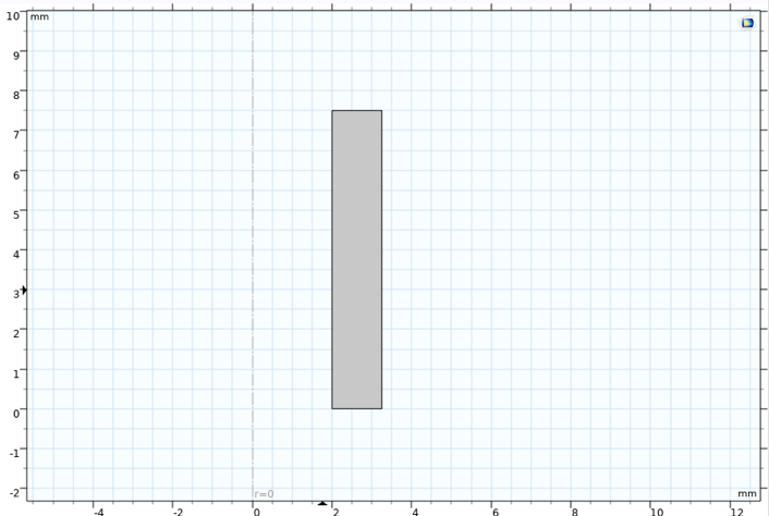
Figure 3. Axisymmetric model of test specimen.
Geometric Model: Fatigue Evaluation
The pressure vessel, representing a realistic case of thermomechanical fatigue, has a total length of 6000 mm, inner radius 950 mm, and thickness 50 mm. This is easily modeled as an axisymmetric model; see Figure 4.
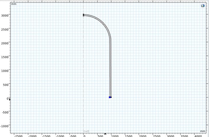
Figure 4. Axisymmetric pressure vessel model.
Mesh: Experimental Comparison
With a very uniform load, the mesh can be quite coarse. Here, it is set to free triangular and a maximum element size of 0.75 mm, as shown in Figure 5.
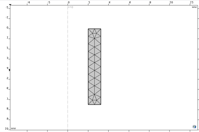
Figure 5. Uniaxial test specimen mesh.
Mesh: Fatigue Evaluation
The pressure vessel model is meshed with a free triangular mesh and a maximum mesh size of 50 mm, shown in Figure 6. It is ensured that there is always more than one element through the thickness, although for the demonstrative purposes of this blog post, it is of little importance.
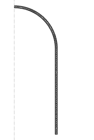
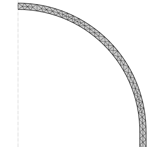
Figure 6. Pressure vessel mesh.
Physics Settings: Materials, Loads, and Boundary Conditions (Experimental Comparison)
The Solid Mechanics interface is used for a thermomechanical fatigue analysis. First, the material must be defined. To enable the necessary models described in the preceding section, we add nodes with viscoplasticity and creep, shown in Figure 7.
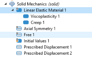
Figure 7. Necessary nodes for material definition.
For the linear elastic, viscoplastic, and creep nodes, the proper material parameters are entered in their temperature-dependent form, as exemplified in the next section.
Since the model is axisymmetric, the only constraint necessary is in the axial direction. The bottom boundary, at z = 0, is constrained in the z direction. The top boundary, however, is assigned the displacement corresponding to the measured strain for the respective load case.
Physics Settings: Materials, Loads, Boundary Conditions (Fatigue Evaluation)
For the pressure vessel case, material setup is identical. Similarly, the symmetry edge at z = 0 is constrained in the z direction. A pressure is applied to the interior wall boundary. This pressure load is a R = 0 load case, with a maximum pressure of 170 bar. The temperature cycling is at a higher temperature than the experimental comparison, with the highest (600°C) at 0 bar, and the lowest (500°C) at 170 bar. The loading rate is 5.67 bar/s.
Study Settings: Experimental Comparison
A time-dependent study is necessary to make use of the creep and viscoplastic material models.
In the isothermal test, the initial cycle is used for comparison. With the strain rate of 0.1%/s, the initial cycle time is 20 s. Output times are chosen at 2.5 s. The time step is set to manual at 0.25 s.
For the anisothermal case, the 50th cycle is used for comparison. With a strain rate of 0.033%/s, the initial cycle time is 60 and the total time is 3000 s. Output times are chosen at 2.5 s, and time step is set to 1 s. The temperature rate is 3.33°C/s.
Study Settings: Fatigue Evaluation
For the pressure vessel analysis, the load and temperature rates are the same as for the anisothermal experimental comparison. The output and time step settings are also identical.
Function and Variable Definitions
Building a model suitable for thermomechanical fatigue analysis is not necessarily complex in and of itself, but there are many aspects to the framework laid out above. Primarily, a framework for consistent variation of temperature and temperature-related material parameters as well as loading is necessary. In COMSOL Multiphysics, this is most conveniently handled by the use of functions and variables. In this section, the method will be outlined using the anisothermal analysis (for experimental comparison).
Parameters
We start by defining global parameters that are unaffected by the solution, including geometry, loading, material creep, and material fatigue parameters (see Figure 8).
Now, the nominal load values (such as temperatures and displacements) can be applied by simple scaling functions that determine the shape of the loading.
Temperature Functions
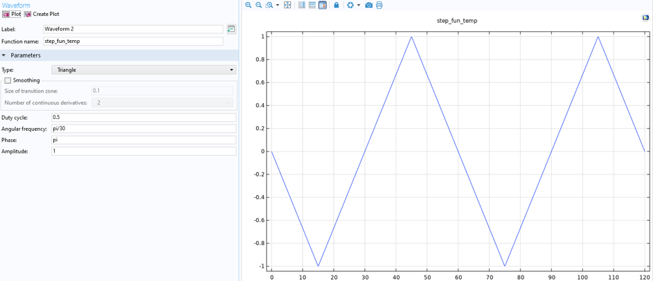
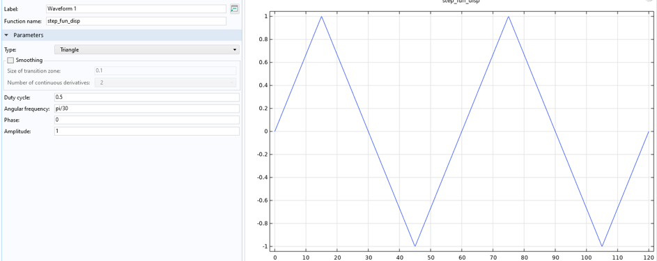
In the isothermal experimental case, the temperature is constant at 400°C. The anisothermal experimental case requires a temperature definition with maximum temperature (500°C) at minimum strain, and minimum temperature (400°C) at maximum strain. This variation is obtained by creating a waveform and analytic function; see Figure 9.
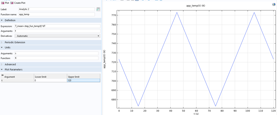
Figure 9. Temperature functions, anisothermal load case.
The temperature is then simply applied as a variable (TempVar) on the model domain; see Figure 10.
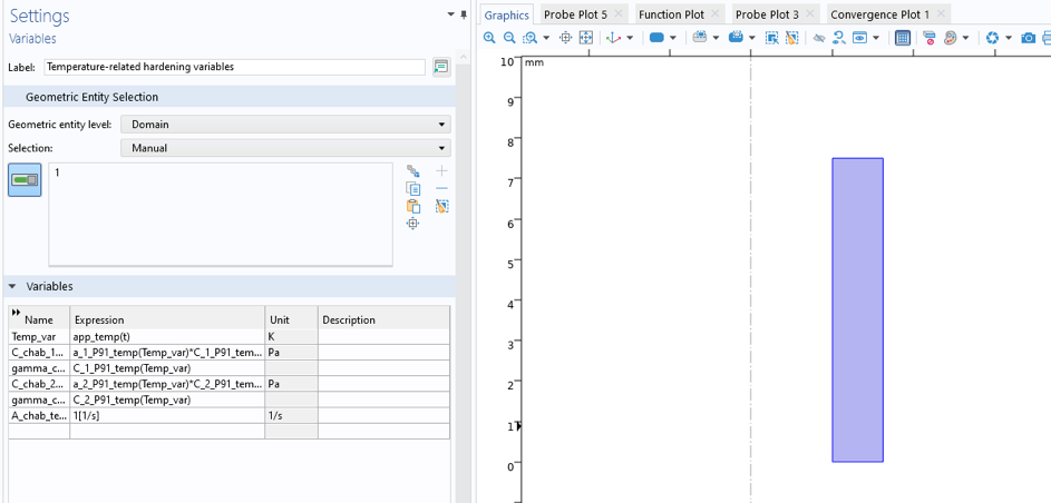
Figure 10. Definition of temperature as a domain variable.
For the pressure vessel case, the temperature is cycled between 500°C and 600°C, as shown in Figure 11. The temperature is likewise represented in the model as a domain variable.
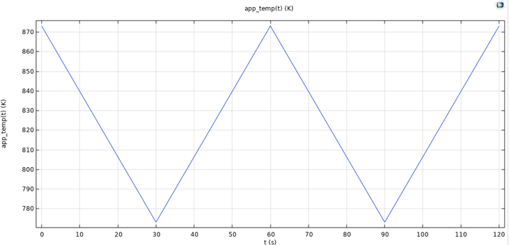
Figure 11. Temperature function, pressure vessel case.
The introduced temperature variable can be used to determine the variation of material properties, but does not take into account thermal expansion. This is of little importance in the experimental case, as the total strain (mechanical and thermal) is machine controlled, but in general, the thermal strain due to thermal expansion should be considered. To do this, a Heat Transfer in Solids physics interface can be included and a pointwise constraint added to enforce the temperature as desired; see Figure 12.
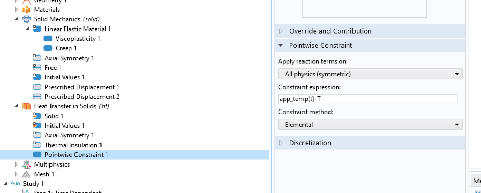
Figure 12. The Heat Transfer in Solids physics interface.
Of course, a homogeneous temperature distribution is seldom realistic. A proper heat transfer analysis can also be used to obtain the temperature field. A reference temperature must be specified for the heat transfer analysis. This is the temperature at which the thermal strains are zero; i.e., a (thermal) stress-free configuration. While this would typically be at room temperature, for fatigue analysis, it is typically the load range and mean, which is of importance. Therefore, in the analysis, the reference temperature is set to 873 K, the max temperature of the cycle.
Load Functions
Similar to the temperature definition, the load (in this experimental case, a displacement) is also defined by two separate functions: waveform and analytic (see Figure 13).
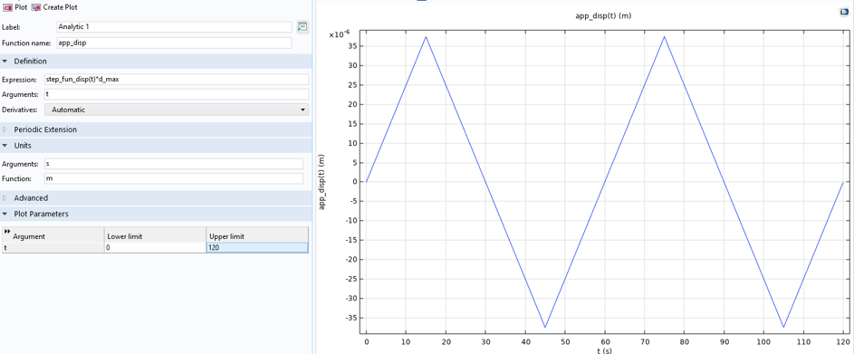
Figure 13. Load functions, anisothermal load case.
This particular figure is specific to the anisothermal experimental case. The strain rates differ between the anisothermal and the isothermal cases. In the latter, the strain rate is 0.1%/s, and in the former, it is 0.033%/s, corresponding to displacement rates of 7.5 µm/s and 2.5 µm/s, respectively. The maximum strain during cycling is 0.5%, which represents an end displacement of 37.5 µm in total. This is related to the gauge length measuring strain over the narrow region of the specimen, 7.5 mm. Note that a half-length model is used; the full length of the narrow region is 15 mm.
In the pressure vessel case, a load function with a peak pressure of 170 bar, load rate 5.67 bar/s, is defined, as shown in Figure 14.
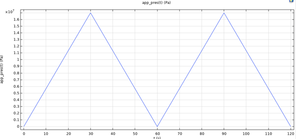
Figure 14. Load function, pressure vessel case.
Material Parameter Functions
The material parameters must have a temperature dependence, and this is most easily obtained by creating an interpolation function with known parameter values at specified temperatures. For example, σsat is defined as in Figure 15.
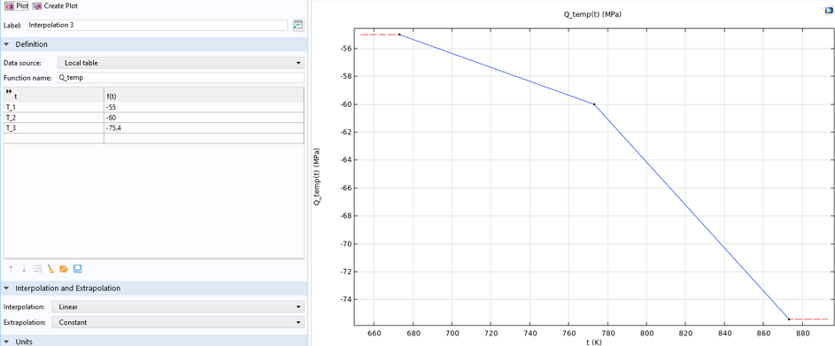
Figure 15. Definition of the function for the temperature-dependent σsat.
The temperature-dependent material parameter is then properly computed by calling this function, using the created temperature variable as the argument. This is shown in Figure 16 for the above parameter as an example, cf. Figure 9. Naturally, the dependent variable T from a Heat Transfer in Solids physics interface may also be used as an argument.

Figure 16. Calling the temperature variable in definition of the material parameter.
The procedure to scale the ultimate tensile strength and fatigue limit with temperature is similar to that outlined above, although a reference value at room temperature is then scaled with a dimensionless reduction factor (because both the ultimate and fatigue strengths are to be scaled). The expression for the analytic function defining the Chaboche S-N curve (cf. Figure 1 and Figure 2) is shown in Figure 17, here defined at room temperature (293 K), as a function of the maximum stress.

Figure 17. Analytic function for the Chaboche S-N curve.
The scaling function UTS_temp_scaling is defined as shown in Figure 18.
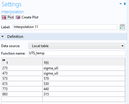
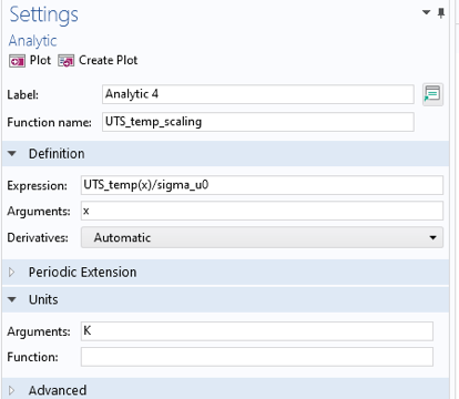
Figure 18. Scaling function for the ultimate tensile strength.
Results: Experimental Comparison
A boundary probe for the average of the first Piola–Kirchhoff stress was created at the top of the model, where the displacement is prescribed. This was extracted and plotted as a function of the applied strain to obtain cyclic stress-strain curves.
Isothermal Testing
The initial cyclic stress-strain curve is shown in Figure 19.
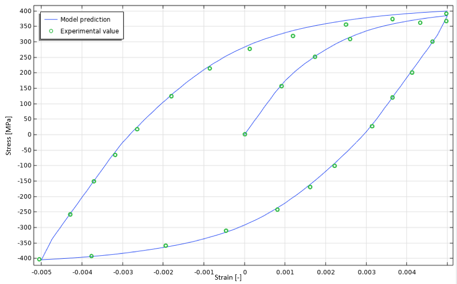
Figure 19. Initial cyclic stress-strain curve, isothermal case.
As expected, the model appears to predict the initial cyclic stress-strain curve well.
Anisothermal Testing
The anisothermal cyclic stress-strain curves are seen in Figure 20.
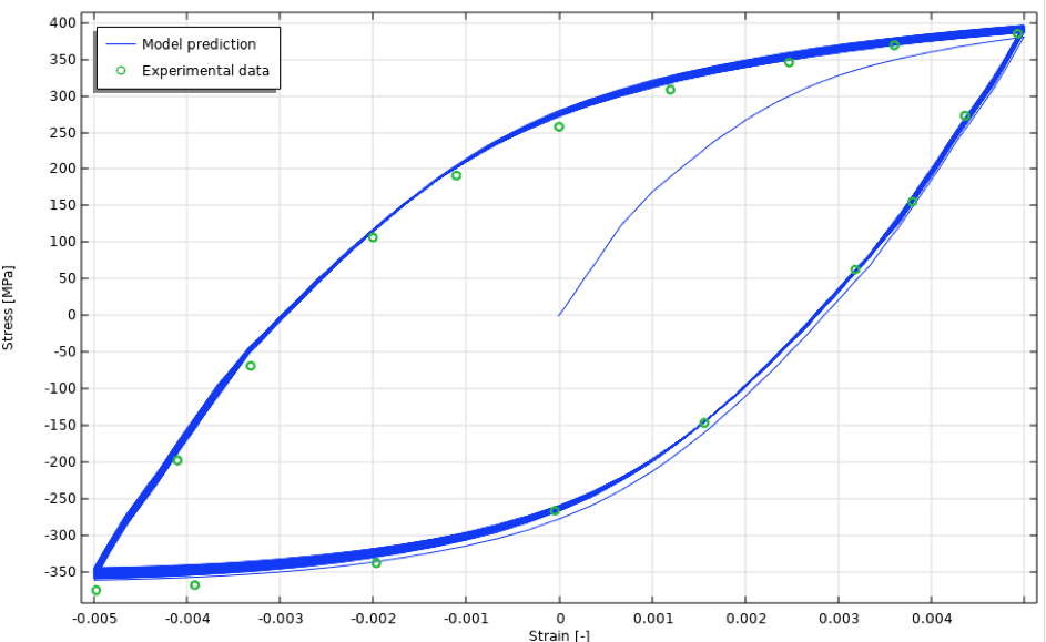
Figure 20. Cyclic stress-strain curves, anisothermal case.
The isolated 50th cyclic stress-strain curve is shown in Figure 21.
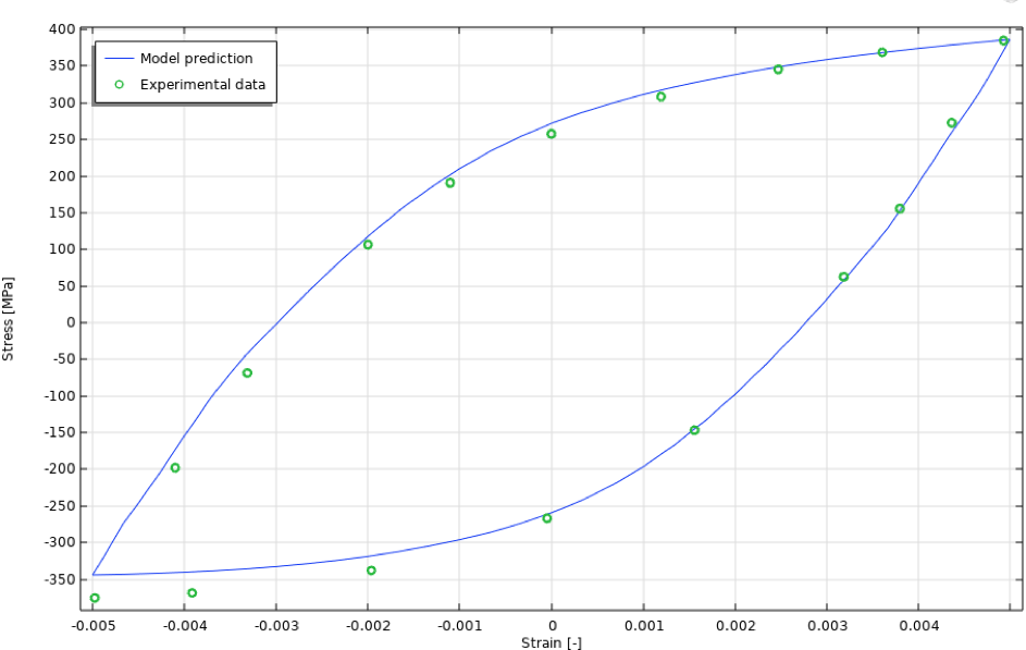
Figure 21. 50th cyclic stress-strain curve, anisothermal case.
Results: Fatigue Evaluation
Stresses and Strains
The von Mises stress at the maximum load (2970 s) and after unloading (3000 s) of the 50th cycle is shown in Figure 22.
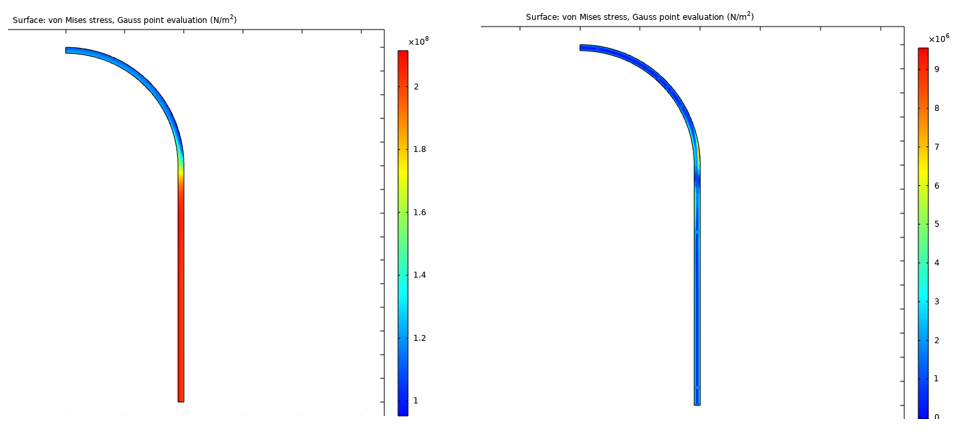
Figure 22. Von Mises stress at maximum load (left) and after unloading (right) of the 50th cycle.
The equivalent viscoplastic and creep strain after the 50th cycle is shown in Figure 23.
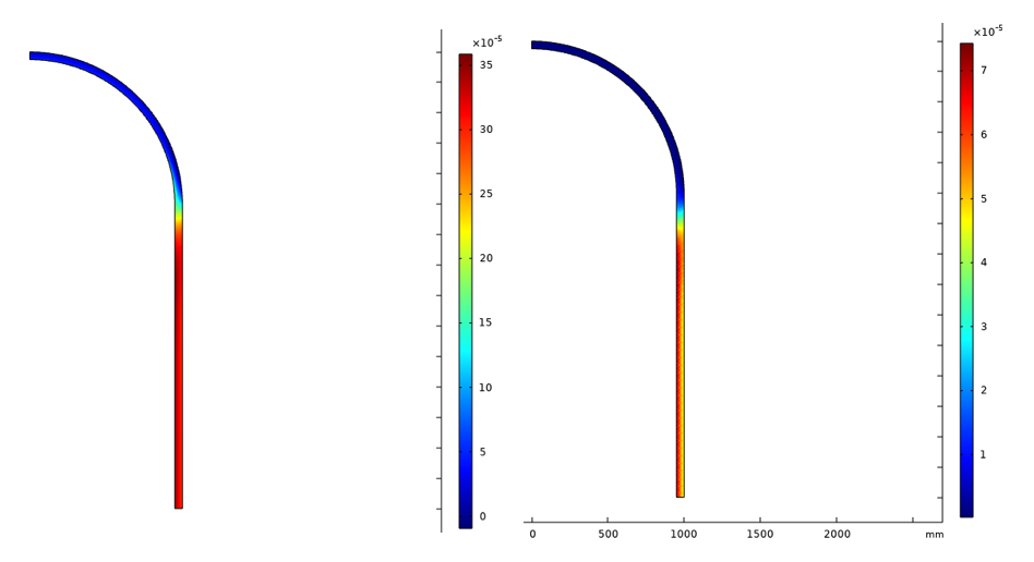
Figure 23. Equivalent viscoplastic (left) and creep (right) strain after the 50th cycle.
A typical behavior of unsymmetric stress cycles is ratcheting, in which the residual strain increases for each cycle. The nonlinear kinematic hardening model accounts for this. Typically, loading cycles with high mean stress tend to increase ratchet strain, and lower mean stress stabilizes the ratchet strain over time. To estimate the number of fatigue cycles without necessarily computing each cycle until failure (see the next section), it is necessary to obtain a stabilized stress-strain cycle. Plotting the maximum von Mises stress for maximum equivalent deviatoric strain in the pressure vessel shows the ratchet strain schematically for two extreme cases in Figure 24.
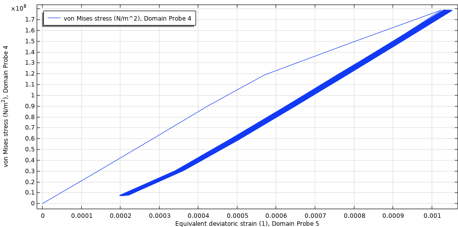
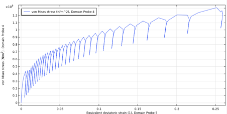
Figure 24. Ratchet strain for low mean stress — maximum pressure 100 bar (left), and high mean stress — maximum pressure 240 bar (right). Both cases are R = 0 loading.
For the low mean stress, the cycle is stabilized almost immediately. For the high mean stress case, the ratchet strain increases for each cycle. In the load case considered here, the maximum pressure of 170 bar, the ratcheting behavior of the first 50 cycles, is shown in Figure 25, extracted at the lower-right model corner. Conservatively, one can also extract the maximum domain values.
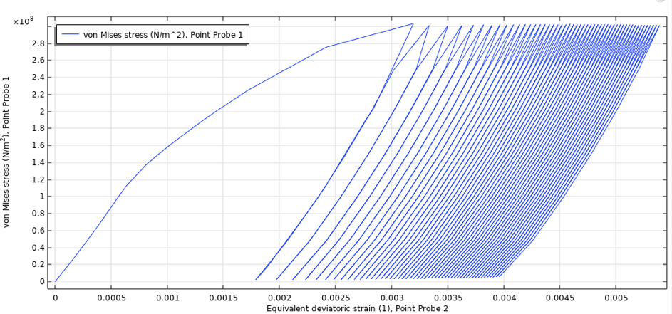
Figure 25. Stress-strain behavior for the pressure vessel, 170 bar maximum pressure, out-of-phase cycling between 500°C and 600°C.
There is a distinct decrease of ratchet strain for each cycle, and the stress-strain curve can be considered stabilized after 50 cycles.
Computed Cycles to Failure
There are several ways to estimate the fatigue life for a component using the equations defined in the preceding sections. The accumulated damage can be computed for each cycle by first finding the effective temperature T* that fulfills
The progression of damage for a cycle can then be computed according to
The total damage is then obtained by summing the damage for each cycle. If these are representative load cycles, the number of such sequences to failure (D = 1) can be obtained. It is also possible to simply compute and sum the damage for each cycle and run the analysis until D = 1. These approaches can be cumbersome, as they require a framework to define and evaluate the variables computed for each cycle. Also, analyzing a component until failure usually requires computing cycles ranging from a few hundred to thousands, even for low-cycle fatigue. For large models, this is usually not viable.
If, however, the component is subjected to a single type of load/temperature cycle, as in the example in this blog post, the number of cycles to failure can then be computed analytically as
One then only needs to compute the mean and maximum stress for a stabilized cycle and evaluate the above expression. First, the stress-strain plot for points at risk of fatigue should be visualized over time to ensure a stabilized cycle. According to Figure 25, the stress-strain cycle appears stabilized.
The mean stress is computed as a derived value of a time average operator of a point solution probe for the maximum stress according to Figure 26: 149.7 MPa.
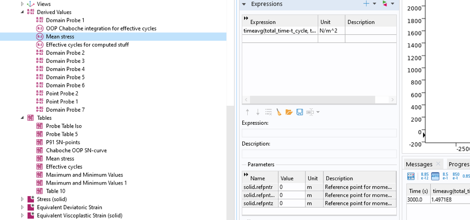
Figure 26. Computation of the mean stress for a stabilized cycle.
The analytical expression for the number of cycles N_{F}^{*} is defined as a function of time, maximum, and mean stress according to Figure 27. This expression differs from the general expression in Figure 17, as it must be used in a time integral.

Figure 27. Definition for a computed number of cycles to failure, as a function of time, maximum, and mean stress.
This is used to compute the number of cycles to failure as a derived value, as shown in Figure 28. The maximum stress is most easily obtained from the probe table: 313 MPa.
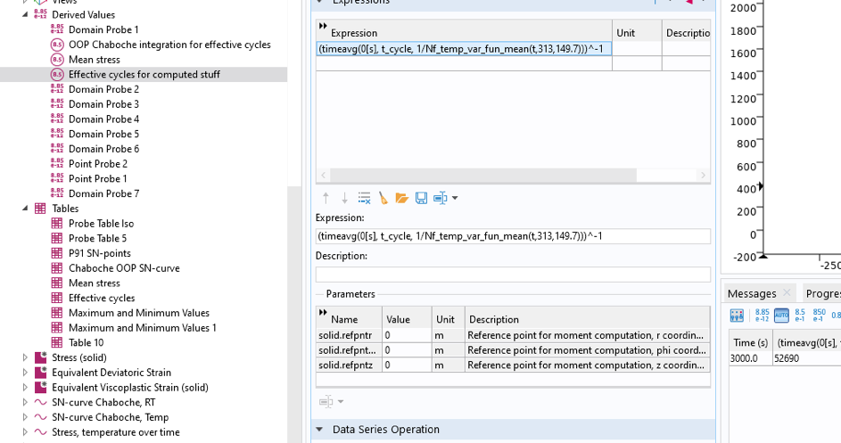
Figure 28. Computation of the number of cycles to failure by use of a Global Evaluation node.
The computed number of cycles to failure is 52,690.
Conclusions and Discussion
Thermomechanical fatigue is of utmost importance in many applications; power plants operating at ever higher temperatures to reduce emissions is just one example. At high temperatures and high loads, temperature-dependent material properties, creep, and thermal strains all affect thermomechanical fatigue.
Using COMSOL Multiphysics, these phenomena can be incorporated by use of the nonlinear material models described in this blog post. Especially important are the hardening parameters, which govern the cyclic stress-strain curve behavior over time. Using the capabilities to define custom functions for temperature and to then make material properties temperature-dependent, makes it possible to use the well-known Chaboche fatigue model to estimate the number of cycles to fatigue failure of a component subjected to simultaneous thermal and mechanical loading. This is easy to do using analytical expressions if the loading/temperature cycle is identical throughout the component life.
For a more complex loading history, it would be necessary to, for each cycle, find an effective temperature representative of thermal and mechanical loading in this cycle. This would then be used to properly scale the relevant material parameters (in this blog post, ultimate tensile strength and fatigue life) used in the function f(\sigma_M, \bar\sigma, D, T^*), and compute the damage for this particular cycle. This incremental process would accumulate damage, and when D = 1, fatigue failure is assumed to occur. For anything with cycles counted in more than a few thousand cycles at most, this is really not a viable approach, as the time required is excessive. Identifying a sequence of representative cycles (a load block) would be a better approach, if possible.
Certain aspects should be noted. The material model used in the referred-to article uses a unified Chaboche viscoplastic model, in which the viscous stress is added to the solution, dependent on the same material parameters used in the Chaboche viscoplastic hardening model. The unified viscoplastic model is not implemented in COMSOL Multiphysics, and the Norton creep law is utilized instead in this blog post. The computed COMSOL Multiphysics results are regardless in good agreement with experimental data. Also, the usage of von Mises stress as a fatigue stress may not technically be a good choice, given its independence of hydrostatic loads. For example, the Sines criterion might be more proper, because the loading is proportional and the direction of principal stress directions can be assumed constant. However, this blog post has little to gain by implementing the Sines criterion.
About the Author
Björn Fallqvist is a consultant at Lightness by Design working with product development based on numerical analysis. He obtained a PhD from the Royal Institute of Technology in 2016, working with developing constitutive models to capture the mechanical behavior of biological cells. His main professional interest and specialization is in the fields of material characterization and using various material models to capture physical phenomena.
References
- S. Natesan et al., Preliminary Materials Selection Issues for. s.l. : Argonne National Laboratory, 2006.
- C.J. Hyde et al., “Thermo-mechanical fatigue testing and simulation using a viscoplasticity model for a P91 steel”, Computational materials science, no. 56, 2012.
- J.L. Chaboche and P.M. Lesne, “A non-linear continuous fatigue damage model”, Fatigue fracture and Engineering Materials Structures, vol. 11, no. 1, pp. 1&ndash17, 1987.
- A.A. Saad et al., “Thermal-mechanical fatigue simulation of a P91 steel in a temperature range of 400-600C”, Materials at high temperatures, no. 28, 2011.
- COMSOL Multiphysics, Structural Mechanics Module User’s Guide.
- X. Feng et al., “Determination of creep properties of P91 by small punch testing”, Materials at high temperatures, vol. 32, no. 4, 2015.
- Y. Gorash and D. MacKenzie, Open Eng, vol. 7, 2017.




Comments (7)
Upendra Gummitha
February 23, 2021Excellent article.
Mohammad Hdaib
May 18, 2021Great blog……
Marwan Nafea
September 16, 2021Nice topic. Is it possible to download the simulation file?
George Scriber
July 28, 2023Wow its really nice article thanks for sharing with us.
Asal Bidarmaghz
June 4, 2024fantastic blog. can the mph file be shared please?
Jan Oredsson
July 20, 2024Hello Björn, this is an interesting post. Thanks for sharing. I am starting a new project to develop a gasket in aluminium which will see temperature cycling between room temperature and 150C.
Lokesh Raj
July 24, 2024Respected Sir
Can you please provide me with the PDF of this simulation? In which the steps are followed to complete this simulation