
When developing a new product or functionality, the first step is typically to understand the functional properties in isolation. To achieve reliable and accurate predictions via mathematical modeling, it is essential that the critical components, test setup, and boundary conditions are specified in great detail. Most engineers, however, would prefer to focus on the critical components rather than “irrelevant” boundary conditions. New impedance boundary conditions in the Acoustics Module of COMSOL Multiphysics help to close this gap.
What Is an Impedance Boundary Condition?
Before answering the above question, let’s first consider the definition of a boundary condition. Heuristically, introducing a boundary condition means that “we know what happens” on the specific boundary. The boundary condition provides additional constraints to the dynamics of the governing equation that is being solved inside the domain. The additions could be, for example, a known vibration velocity, a sound hard wall, or a symmetry plane. Imposing such constraints, COMSOL Multiphysics looks for a solution that satisfies the acoustical dynamics and the boundary condition.
Impedance models are really models of a “full flow”, that is, a condition imposed simultaneously on the acoustic pressure and acoustic velocity, defining a given relation between the two elements. Such relations are known in some idealized cases. Introducing an impedance condition essentially forces a certain idealized acoustic behavior. An impedance boundary condition is therefore a powerful yet simple condition that is applied to situations in which the idealized dynamics are obvious. Microphone cavities with well-known membrane dynamics, acoustics in long pipes, and plane-wave acoustics at porous surfaces are some relevant examples.
Mathematically, the specific impedance boundary condition specifies a linear relation between pressure p and velocity v
(1)
where Z_\textrm{s} is the so-called impedance containing the dynamics (SI unit: Pa*s/m). The most advanced impedance models are given in the frequency domain. As such, Z_\textrm{s} is generally a frequency-dependent parameter, Z_\textrm{s}=Z_\textrm{s}(\omega).
Rather than specifying a specific impedance that relates the velocity to the pressure at every single point (as in Eq. (1)), the acoustic impedance Z (SI unit: Pa*s/m^3) relates the pressure acting on a surface to the volumetric flow Q rate at that surface, such that
(2)
Finally, we have the characteristic specific impedances Z_\textrm{c} defined for traveling waves. These types of impedances relate the particle velocity and pressure at every point as the wave moves through the domain, making them useful low-order models for an infinite domain. One example is the well-known relation for plane traveling waves, Z_\textrm{c}=\rho c.
New Impedance Models in the Acoustics Module
The Impedance boundary condition — part of the Acoustics Module in COMSOL Multiphysics — features several new models that are directly applicable to a range of acoustics applications. All of the additions contain frequency dependencies and are available only in the frequency domain. (To define an impedance boundary condition in the time domain, you can use the User defined impedance boundary condition.) The table below describes the models, included under the Impedance boundary condition in the Pressure Acoustics physics interface.
| Name | Description | Applications |
|---|---|---|
| RCL | Lumped-parameter circuit element models, allowing for any combination of an acoustic resistance (R), compliance (C), and inertance (L). |
Electroacoustics: Models of microphone membranes, transducers, etc. for mobile devices and consumer electronics.
Acoustic-solid interactions: Simple models of the mechanical behavior of elastic materials and solids. In general: Model the behavior of any surface that can be modeled as a simple resonator circuit. |
| Physiological | Experimentally verified models of the human ear and human skin. |
Hearing aids: Appropriate boundary conditions for hearing aids used within the ear.
Head sets, mobile devices, ear phones: Realistic acoustic loads for the working conditions of such consumer devices. Human skin: Simulations where the human body is part of the simulation domain. |
| Waveguide end impedance | Models of the acoustics at waveguide ends, with options for flanged and unflanged configurations. | Long pipes and ducts: Used to truncate the simulation domain when pipes and ducts end. The relations are good approximations when the propagating waves are plane waves. |
| Porous layer | General model of normal-incidence acoustics on a layer of porous material backed by a hard wall. | Room acoustics: Simple boundary condition for room acoustics simulations with sound-absorbing layers. |
| Characteristic specific impedance | Idealized models of traveling-wave acoustics of infinite domains for plane, cylindrical, and spherical waves. | Infinite domains: Crude models of an infinite domain, assuming that the acoustic radiation from the region of interest can adequately be approximated as plane waves, cylindrical waves, or spherical waves. The radiation boundary conditions are more elaborate versions of this condition. |
As the screenshots below indicate, toggling between the array of impedance models is quite easy. For the more complex options, we have included an illustration to offer a better description.
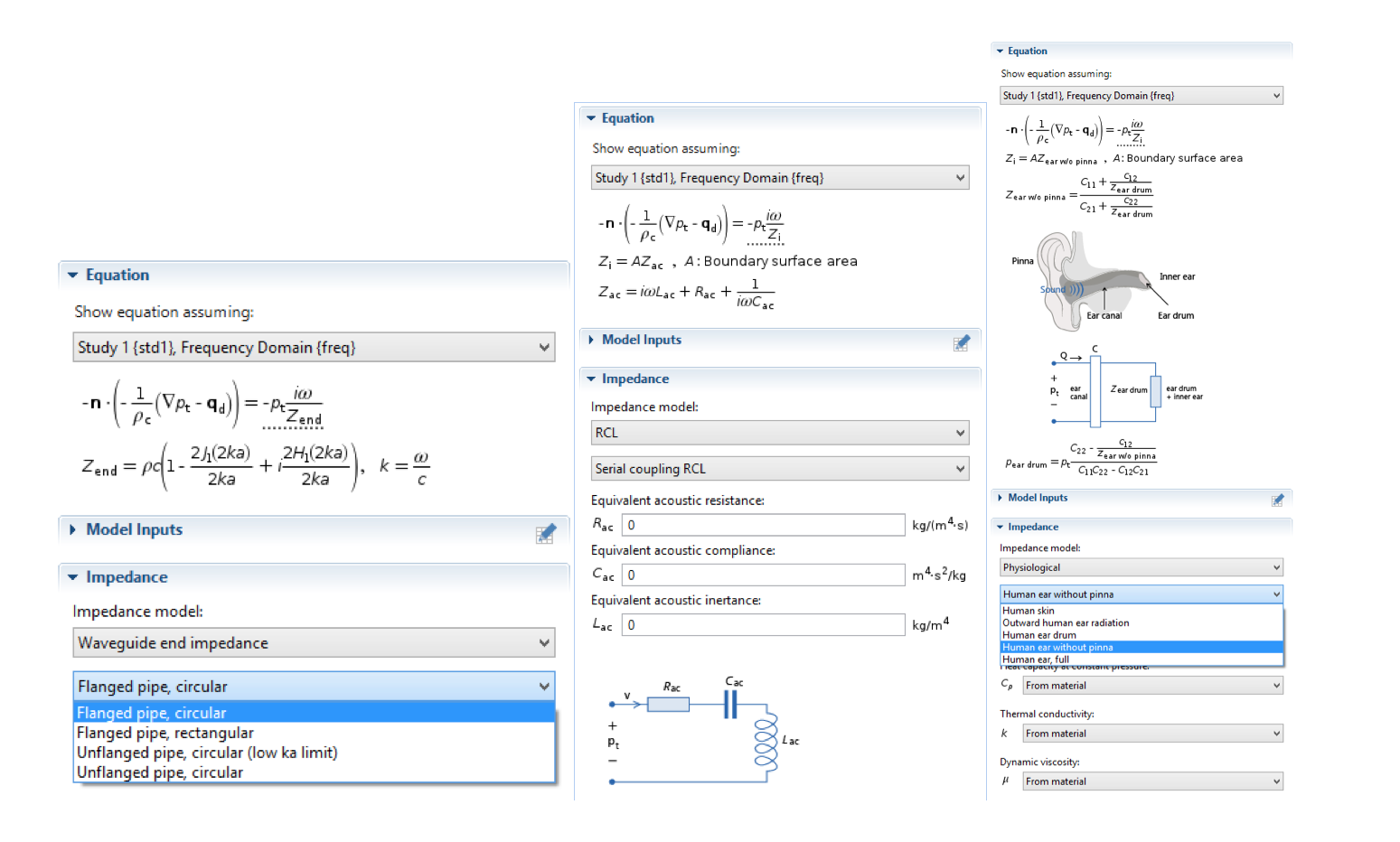
The user interface (UI) for some impedance models, including the Flanged pipe, circular model; Serial coupling RCL model; and Human ear without pinna model.
Working with Impedance Boundary Conditions in Acoustics Simulations
In the rest of the blog post, we will walk through a few examples that demonstrate how to exploit the RCL functionality option in the impedance boundary conditions. The first model focuses on the use of an RCL circuit to represent a measurement microphone. The last two examples are based on the same system, with a complex COMSOL Multiphysics model treated as an “experiment” in which certain parts (a submodel) can be parameterized by an impedance. In the first case, the impedance is given as an interpolation function. In the second case, an RCL model is fitted to the data using optimization.
An RCL Condition in Electroacoustics
We can begin by considering a case in which parameters for an impedance boundary condition are known. Such a situation is common in electroacoustics, as lumped-parameter values are often specified for devices.
In many engineering branches, acoustics included, lumped-parameter modeling is a recognized strategy for establishing useful models without spatial resolution. In the new Impedance boundary condition, a general framework for simple lumped-parameter models is available under the RCL option. Let’s use the example of a simple microphone, as demonstrated in our lumped receiver tutorial. Here, the behavior of a receiver (miniature loudspeaker) is analyzed, with a microphone placed at the opposite end to read out the signal.

Model geometry of a receiver (miniature loudspeaker) placed in a test setup.
To model the microphone, we use a serial RCL impedance condition
(3)
C is the compliance of the microphone (a measure of the air volume behind the diaphragm as it is pushed back), R is the losses of the system (thermoviscous damping), and L is the acoustic mass of the diaphragm. The condition is applied evenly across the entire end of the outlet, implicitly neglecting variations in diaphragm displacement at different radial coordinates that would occur if a full microphone model was included.
Compared with experimental measurements, the model offers excellent predictions across a broad frequency band using the simple boundary condition in Eq. (3) for the microphone. The impedance provides a boundary condition with sufficiently realistic dynamics, keeping the focus on the detailed modeling of the receiver and other elements.
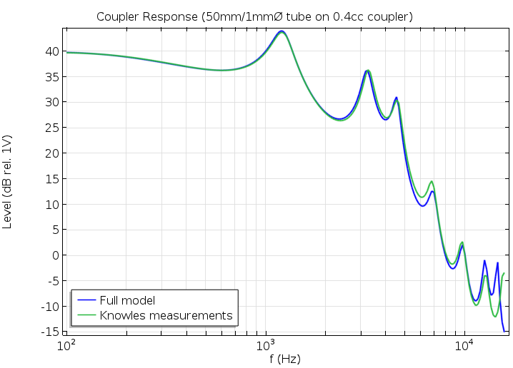
A plot comparing pressure inside the coupler region.
How to Model a Subcomponent Using an Impedance
Shifting gears, we’ll now look at how to extract an impedance model in order to represent a complex subcomponent. You can download the model presented here from our Application Gallery.
The example involves a simple muffler-like system (or it could be a part of a muffler) consisting of a long tube with a 2D axisymmetric Helmholtz resonator (see figure below). A plane wave of amplitude p_\textrm{in} is incident at the inlet with radiation conditions applied at the inlet and outlet. Noticeable viscothermal damping is present in the narrow neck of the Helmholtz resonator. Because of such losses, the Pressure Acoustics interface is insufficient and the full model uses the Thermoacoustics interface in that region. In the main parts of the duct, the Pressure Acoustics interface suffices. The model utilizes the Pressure Acoustics and Thermoacoustics interfaces, along with the Acoustic-Thermoacoustic Boundary multiphysics coupling.
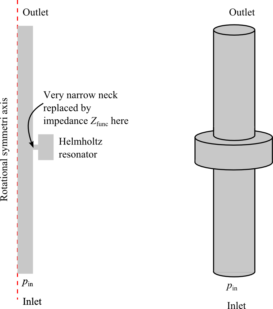
Muffler-like system with a Helmholtz resonator. The schematic on the left corresponds to the 2D axisymmetric geometry implemented in COMSOL Multiphysics. Notice the very narrow neck into the resonator, which is responsible for viscothermal losses.
User-Defined Impedance Given by an Interpolation Function
When moving from component simulation to system simulation, it can be advantageous to lump certain parts or full components (i.e., solving the thermoacoustic model in the current resonator is computationally expensive). To do so, we can replace the Thermoacoustics submodel (the Helmholtz resonator) with an impedance boundary condition, applying the condition to the area where the inlet to the neck is located. In this way, it is possible to simulate the whole model with only the Pressure Acoustics interface.
First, we extract the effective impedance Z_{\textrm{func}} at the neck from the full model. We compute the ratio of the average inlet pressure to the average inlet velocity, as
(4)
The figure below illustrates the real and imaginary parts of Z_{\textrm{func}}. The data is used to create two interpolation functions for Z_{\textrm{func}}: one for the real part (Zfunc_real) and one for the imaginary part (Zfunc_imag). The functions contain all of the information about the impedance and can be called from inside the User Defined impedance boundary condition by writing: Zfunc_real(freq)+i*Zfunc_imag(freq). Using the impedance, we set up a simplified version of the model with only the Pressure Acoustics interface. The Helmholtz resonator is no longer included in the setup, but it is represented by the impedance.
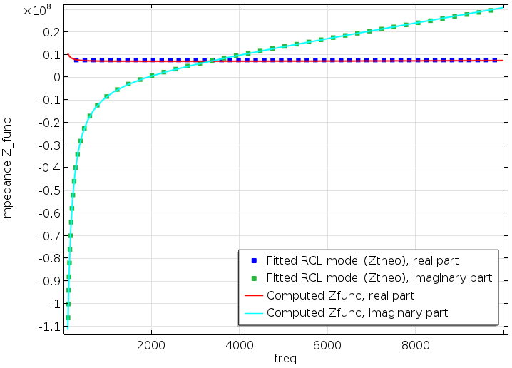
Resonator impedance Z_{\textrm{func}} as obtained via Eq. (4) from the fully coupled model. The points indicate the best fits of Eq. (6) to the data given by the solid lines.
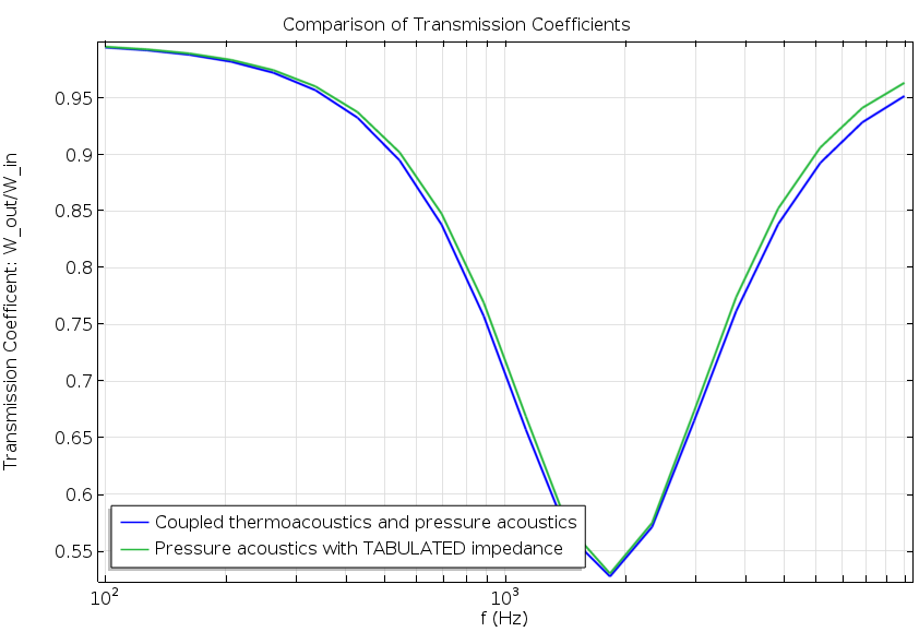
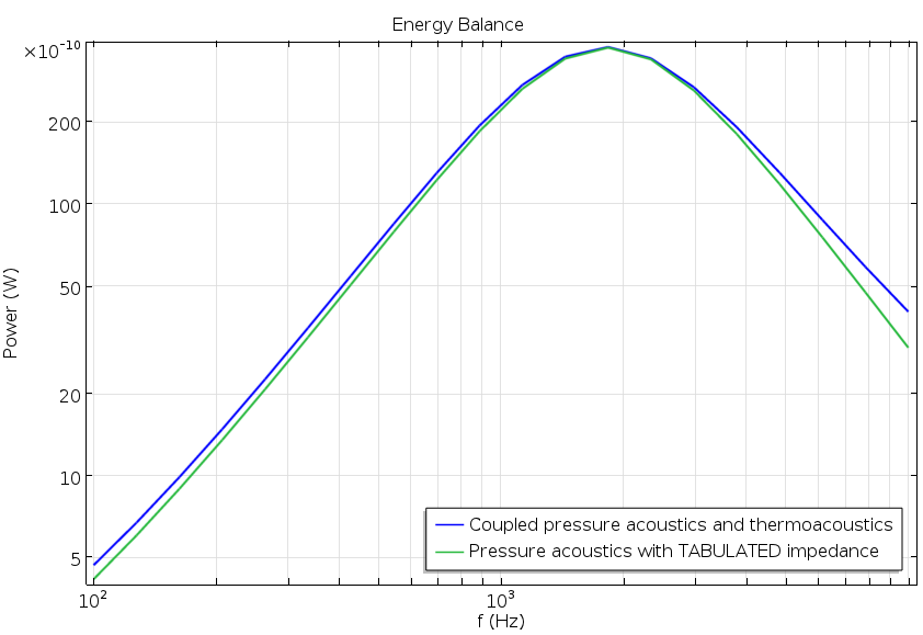
To evaluate the performance of the simplified model, we compute the transmission coefficient \tau across the main tube. The transmission coefficient is defined as the ratio of the transmitted power (W_{\textrm{out}}) relative to the incident inlet power (W_{\textrm{in}}). We also plot the “energy balance”, that is, the dissipated energy in the system. This is given as the difference between the incident and reflected and transmitted power,
(5)
where W_{\textrm{ref}} is the reflected power.
The results are depicted in the following two figures. Good agreement is shown in both of the graphs, with little difference between the full model and the simplified model using the interpolated impedance. Shorter solution times are an added benefit, as the simplified version takes only 3 seconds to solve (the fully coupled model took 25 seconds). While the numbers are hardware-dependent, they do reflect the computational efficiency of removing the need to solve the thermoacoustic model in the resonator.
Transmission coefficient plot (left) and power balance plot showing the dissipated energy (right).
In most realistic situations, however, it is not particularly advantageous to first solve a complicated version of a model and then reduce it. Single subcomponents can be modeled individually and characterized. The detailed impedance models of the complex subcomponents derived from full models should be kept in a library and called upon when necessary. COMSOL Multiphysics has functionality to support such a practice: Tabulated values of the results from complex subcomponents can be saved to files and brought in as needed.
A Fitted RCL Model Using Optimization
In cases where a priori knowledge is used to deduce the mathematical form of the impedance, or when the data obviously lends itself to simple mathematical forms, the preferred route may be to fit a simple theoretical model to the full detailed COMSOL model. In the former case, the parameter values of the impedance model reflect characteristics of the underlying physics and offer insight into the system. For instance, if the data is described well by an RCL-type model, such as Eq. (3), the resonance frequencies are immediately available.
We will illustrate the steps for fitting a theoretical model to an impedance boundary condition. The Helmholtz resonator has a moving acoustic mass (the air in the neck), a compliance (the compressible air in the resonator volume), and losses (the thermoviscous losses). Thus, a good model across the entire frequency range is
(6)
where R_{\textrm{func}}, C_{\textrm{func}}, and L_{\textrm{func}} are unknown parameters to be fitted. The Optimization Module is used to perform a best fit of Eq. (6) to Z_{\textrm{func}} with the objective function \left| \left( Z_{\textrm{theo}}- Z_{\textrm{func}} \right)^2 \right|. The following fitted parameter values are obtained
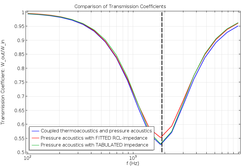
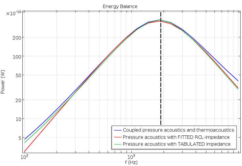
The values are entered directly into the Impedance boundary condition via the RCL option. (For general theoretical models, the User defined option can be used as it accepts any model, no matter the level of complexity.) Using only the Pressure Acoustics interface and the RCL impedance model, we once again compare the results from the new simplified version to the fully coupled model. We plot the transmission coefficient \tau and the power balance from Eq. (5).
Transmission coefficient (left) and power balance (right) plots. Results are shown for the simplified model (red), the full impedance model (green), and the fully coupled model (blue). The latter two results were presented in this earlier figure.
We again observe good agreement for both metrics across the entire frequency range. The high-frequency response provides a slightly better representation of the fully coupled model than in the initial example, while the situation is opposite for low frequencies.
As mentioned earlier, simple, well-known boundary impedance models can be used to obtain even more insight about the system. Let’s apply such an approach to our present simple muffler case.
The resonance frequency for series-coupled RCL models, such as Eq. (6), is given by f_{\textrm{res}}=\frac{1}{2 \pi \sqrt{C_{\textrm{func}} L_{\textrm{func}}}}. It is, therefore, expected that the optimal muffler working conditions (lowest transmission coefficient) will be achieved at the frequency
Indeed, this is found to be the case. Dashed vertical lines indicate the resonant frequency in the figures above, predicting the minimum transmission coefficient very well.
If you have any questions, please contact us.




Comments (0)