Simulating Natural Convection in Air with COMSOL Multiphysics®

Natural convection is a type of heat transport found in engineering applications of all sizes. For instance, this phenomenon helps maintain a reasonable temperature in both small electronic devices and large buildings. No matter the application area, design engineers can use the COMSOL Multiphysics® software to model natural convection in air for both 2D and 3D geometries.

Transporting Heat with Natural Convection

The process of natural convection, also called buoyancy flow or free convection, involves temperature and density gradients that cause a fluid (like air) to move, leading to the transport of heat. Unlike forced convection, no fans or external sources are needed to generate fluid flow — just differences in temperature and density.

Natural convection in air has a wide range of applications in various industries. In the electronics field, this phenomenon dissipates heat in devices, which helps prevent them from overheating. Additionally, structures like solar chimneys and Trombe walls take advantage of this heat transport method to heat and cool buildings. The agricultural industry also depends on natural convection, which helps in the drying and storage of various products.

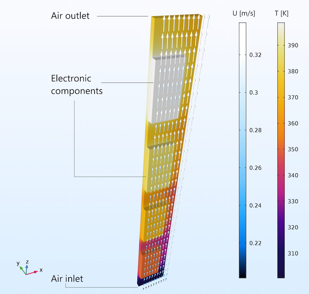
Natural convection of air through vertical circuit boards.

With the COMSOL Multiphysics® software, it is possible to study natural convection in air for both 2D and 3D models. Let’s take a look at one example…

Simulating Natural Convection in Air

The Buoyancy Flow in Air tutorial shows how to model natural convection in air for two geometries:

1. 2D square
2. 3D cube

In both cases, all of the edges are insulated except for the left and right sides, which are set to a low and high temperature, respectively. The temperature difference (around 10 K) leads to density gradients in the air, generating buoyancy flow. Note that the cube has more sides than the square, which influences how the air flows.

To simplify the model setup, there are a couple of built-in features in COMSOL Multiphysics that we can use. First up is the predefined Nonisothermal Flow interface, which couples fluid dynamics and heat transfer in the model. We can also use the Material Library to easily determine the thermophysical properties of air.

Next, we can estimate the flow regime by computing the Grashof, Rayleigh, and Prandtl numbers. The Grashof and Rayleigh numbers suggest that the flow is laminar, with a velocity of around 0.2 m/s. As for the Prandtl number, it indicates that viscosity doesn’t influence the buoyancy of the air and that the shear layer thickness is about 3 mm.

For more details on estimating the flow regime, download the model documentation from the Application Gallery.

Note: The Buoyancy Flow in Water tutorial model demonstrates a similar model setup with water instead of air.

Examining the 2D and 3D Simulation Results

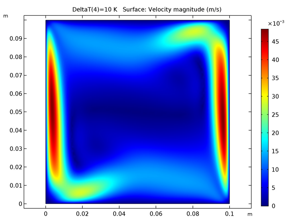
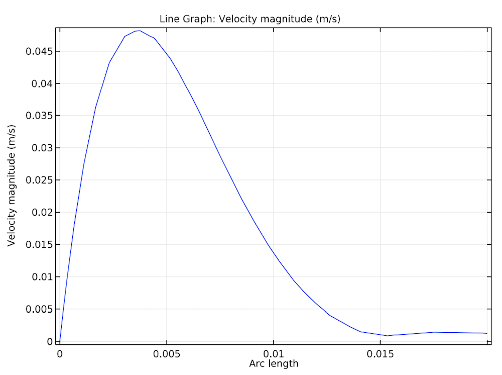
Let’s take a look at the results, starting with the velocity magnitude of air in the 2D square. In the left image below, we see that the velocity increases as the air nears the left and right edges, with a maximum velocity of 0.05 m/s. While this is a bit lower than the estimated velocity calculated using the Grashof and Rayleigh numbers, it is still in the same order of magnitude. Further, the shear layer thickness (3 mm) corresponds with the estimate from the Prandtl number.

The velocity magnitude (left) and velocity profile (right) of air in the 2D square.

As shown below, the results for the velocity magnitude in the 3D cube are similar to those for the 2D square.

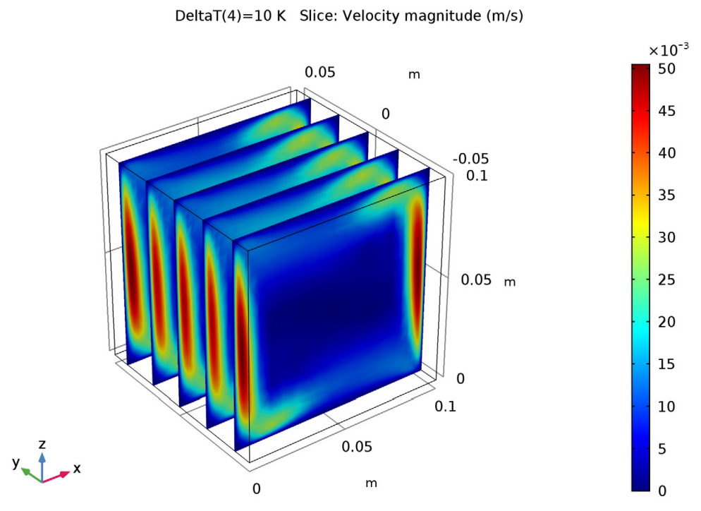
Velocity magnitude in the cube.

Next up, let’s look at the temperature results for the 2D geometry. A single convective cell fills the square, with the air flowing around the edges. We see that the flow of air is faster at the left and right sides, where the temperature differences are the greatest.

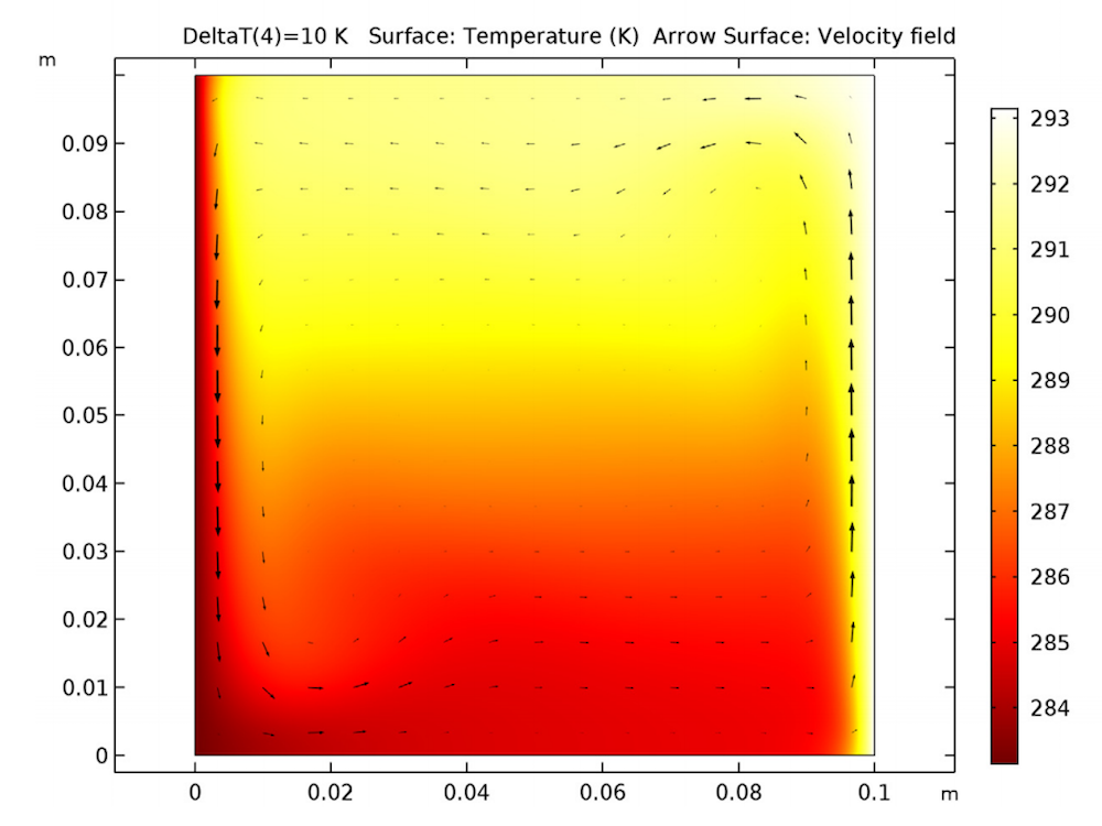
The temperature field in the square.

The 3D results show a slightly different scenario. There are small convective cells in the cube at the corners of a vertical plane perpendicular to the heated sides. As mentioned, this difference is likely due to how the front and back sides in the cube affect the airflow.

The temperature and velocity fields in the 3D cube.

Next Step

The model geometries in the Buoyancy Flow in Air tutorial are rather simple, but the example provides you with a solid foundation for modeling natural convection in more detailed models that represent real-world applications.

For more details about this example, go to the Application Gallery via the button above. From there, you can download the MPH-file and step-by-step instructions on how to build the model.