
In a previous blog post, we discussed the mechanisms used for selecting the time step and the discretization order for the BDF time-stepping scheme. These mechanisms are designed to guarantee solution accuracy according to the prescribed tolerances with a tradeoff between efficiency and robustness. In this follow-up, we explain which measures should be taken for improving the simulation efficiency where small automatic time steps are encountered. We’ll look at some examples and discuss which solver settings can be adjusted.
Tracking the Time Step and Discretization Order in the Solver Log
When inspecting the solver log of a time-dependent simulation using the BDF time-stepping scheme, the order of the BDF scheme and the time step varies according to the mechanisms described in the previous blog post. We might find ourselves in one of three potential scenarios:
Scenario 1: Varying Time Step and Discretization Order
From the solver log, we find that NLfail = 0 and Tfail = 0 (no failures are recorded for the time-dependent and algebraic solvers), but both the time step and discretization order are varying.
This is a typical scenario and expected behavior for well-behaved models. When the local truncation errors are small, the time step size increases. An increasing discretization order indicates smooth solutions with monotically decaying higher-order time derivatives. Effects of a nonlinearity are taken care of by the algebraic solver and are reflected by some extra algebraic solver iterations or some extra Jacobian updates, but this does not affect the time stepping in any other way.
Typically, but not always, adjustments for the solver settings are not required. However, there is always a risk that the tolerances are too large for the problem at hand, and that some effect or detail in the solution is missed; that the solution is underresolved. This can happen, even when the error estimates are fulfilled for all time steps. Therefore, it is always a good idea to reduce the tolerances and repeat the simulation. This should result in smaller time steps and improve the solution accuracy at the price of a higher CPU time. Also, note that the algebraic termination criteria is directly related to the tolerances for the time solver, so a too-large tolerance risks influencing not only the time discretization error but also the error from terminating the algebraic problem iterations.
Therefore, in some cases, lowering the tolerances can result in a better resolution of the details of the solution and lead to smoother error estimates, which in turn gives rise to larger time steps. This is somewhat counterintuitive, since lowering the tolerance in these cases also leads to more effective (faster) time stepping.
Example: One-Dimensional Viscous Burgers’ Equation
Let’s consider the Burgers’ equation
with a smoothed-out step function as the initial value and diffusion coefficient c=0.001, convection coefficient \alpha=1, and nonlinear convection coefficient \beta=1.
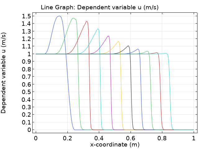
We solve using a quadratic Lagrange element discretization in the interval (0,T] \times (0,1) with homogeneous Dirichlet boundary conditions using the default solver settings. Due to the nonlinearity, a viscous shock profile is forming. We conduct a mesh convergence analysis first, in order to identify a reasonable mesh size and tolerance.
A reference solution u_{\rm ref} is computed for T=0.15 with Maximum element size h_{\rm max} = 1e-6 (corresponding to 2e6 degrees of freedom), Relative tolerance R=1e-5, and 855 time steps. We determine the maximum point errors e_{P1} := {\rm max}_{t \in (0,T]} |u(t,0.2)-u_{\rm ref}(t,0.2)|, e_{P2} := {\rm max}_{t \in (0,T]} |u(t,0.35)-u_{\rm ref}(t,0.35)|, and the integral error e_I := {\rm max}_{t \in (0,T]}\int_0^1 |u(t,x)-u_{\rm ref}(t,x)|dx. If the mesh is too coarse or the Relative tolerance is too large, there are visual spikes in the solution (see the red values in the table below; spikes are reflected by e_{P2} only).
| R=0.01 | R=0.001 | R=0.0001 | R=0.00001 | |||||||||||||
|---|---|---|---|---|---|---|---|---|---|---|---|---|---|---|---|---|
| h_{\rm max} | # | e_{P1} | e_{P2} | e_I | # | e_{P1} | e_{P2} | e_I | # | e_{P1} | e_{P2} | e_I | # | e_{P1} | e_{P2} | e_I |
| 1e-2 | 106 | 1.5e-2 | 4.9e-1 | 8.1e-3 | 195 | 5.5e-3 | 1.6e-1 | 1.8e-3 | 272 | 9.3e-4 | 1.6e-1 | 1.7e-3 | 380 | 1.6e-3 | 1.6e-1 | 1.7e-3 |
| 1e-3 | 109 | 2.7e-2 | 4.2e-1 | 8.0e-3 | 246 | 6.0e-3 | 1.6e-1 | 1.8e-3 | 508 | 1.7e-3 | 2.1e-3 | 8.3e-5 | 904 | 9.0e-7 | 1.8e-4 | 3.7e-6 |
| 1e-4 | 109 | 2.7e-2 | 4.2e-1 | 8.0e-3 | 246 | 6.0e-3 | 1.6e-1 | 1.8e-3 | 461 | 1.7e-3 | 1.2e-3 | 8.3e-5 | 833 | 1.2e-8 | 3.8e-7 | 1.4e-6 |
| 1e-5 | 109 | 2.7e-2 | 4.2e-1 | 8.0e-3 | 246 | 6.0e-3 | 1.6e-1 | 1.8e-3 | 510 | 1.7e-3 | 1.3e-3 | 8.3e-5 | 855 | 9.8e-9 | 6.3e-8 | 3.5e-9 |
# denotes the number of time steps.
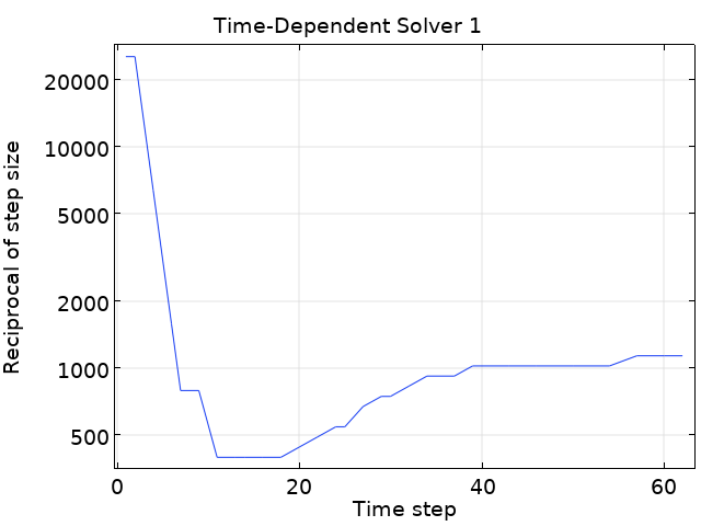
From the first columns, we can see that a finer mesh cannot reduce the error if the Relative tolerance is too large. The default tolerance needs to be decreased. We also find that decreasing the tolerance alone does not reduce the error when the mesh is too coarse. Even for smaller tolerances, there is a saturation of the error for a specific mesh size. The number of time steps increases when the tolerance is lowered (note that the absolute tolerance is coupled to the relative tolerance). In the course of the simulation, the time steps drop in size for the first couple of steps and they slightly increase until the end. The largest admissible tolerance is R= 0.0001 in this example. For a sufficiently small tolerance, the error magnitudes depend on the mesh resolution. Note that a finer mesh does not give more time steps.
We further find that by decreasing the Tolerance factor from 1 to 0.1, we can decrease the number of time steps taken (not shown in the table). The reason is that the algebraic solver is subject to a lower tolerance with this setting, and there is less pollution of the transient error by the algebraic error. From the solver log, we find that the BDF order remains at 5 until the end of the simulation (otherwise, it decreases due to the algebraic error). The total measured error remains on approximately the same level as when less time steps are computed. This is a nice example to demonstrate that tighter tolerances can give a more efficient (faster) time stepping. It is also a nice example of how the spatial and temporal errors both need to be considered when solving PDEs.
For this example, there are no failures recorded in Tfail or NLfail, and the BDF order quickly increases from 1 to 5 and keeps varying between 2 and 5 later (when the Tolerance factor is not reduced). For this simple example, the algebraic solver is working well. We can also switch from Constant (Newton) to Automatic (Newton) and obtain the same behavior, even if this solver is using a much more expensive Jacobian update strategy (every iteration). For the Automatic highly nonlinear (Newton) solver, however, we find that NLfail quickly increases, and we get a failure in every second step on average. The reason is that this solver starts with a conservative damping factor and will typically not converge in 4 iterations, even for benign problems. It is illustrative to see how these failures lead to a reduction of the time step to around 1e-5s instead of 1e-3s. (100 times more steps are needed!) This is a dramatic deterioration of the performance of the time stepping. The failures for the nonlinear solver and the smaller time steps can be fixed by increasing the Maximum number of iterations for the Fully Coupled solver from 4 to 6 (so that the algebraic solver is given a chance to do its job).
Frequent failures of the nonlinear solver are also observed for the choice Constant (Newton) with Damping factor \omega=0.5 and Maximum number of iterations limited to 2. We find that the time steps become smaller than before. When increasing the Tolerance Factor to 10, there are failures recorded in NLfail and Tfail. It might look odd to mess up the algebraic solver, but it serves as an illustration of a badly set up algebraic solver spoiling the time-dependent solution process. These errors also persist when \beta=0 is used (a linear problem). Increasing the Tolerance factor further gives only errors in Tfail (the algebraic solver accepts large errors).
Scenario 2: NLfail Is Greater than Zero
From the solver log, we find that NLfail > 0.
The time-dependent solver computes the solution to an algebraic problem, possibly nonlinear, at each time step. Every time the algebraic solver fails, the NLfail column is incremented. The Jacobian (or Jacobians) for the algebraic iterations is relatively expensive to compute. Therefore, by default, the reevaluations of the Jacobian are done as seldom as possible (Jacobian update is Minimal). If the algebraic solver does not converge, the time step is reduced, the Jacobian (or Jacobians) is recomputed, and the algebraic problem is solved again. This is rather expensive. Notice that since the time step is part of the Jacobian matrix, the Minimal Jacobian strategy can also cause linear problems to fail to converge.
If the algebraic solver fails because the time step is becoming too large, and it happens over and over again, then we can improve the situation by enabling the Nonlinear controller within the Time Stepping settings, which allows for more conservative time step control — especially for highly nonlinear problems.
If the algebraic solver still fails, increase the Maximum number of iterations. Secondly, change Jacobian update to On every iteration (or at least to Once per time step). Next, we can attempt different acceleration or robustification methods. Anderson Acceleration is useful together with the Segregated algebraic solver. It might help to switch to the Fully Coupled solver instead (if the amount of available memory permits). For the Fully Coupled solver, lowering the constant damping factor or using the Automatic damping method can be helpful.
If the algebraic solver still does not converge, we can change the Solver Log to Detailed and thereby get error estimates for the individual dependent variables (as of COMSOL Multiphysics® version 5.5). This information is not only printed to the Log view but also displayed in a separate Convergence Plot window. With this information, we can track down which variable is dominating the algebraic error, which gives us insight into the convergence problem. Notice that the error weights for a dependent variable are affected by both the scaling and the choice of absolute tolerance for that variable.
Another important parameter directly influencing the termination of the algebraic solver is the Tolerance factor. A value of 1 means that the termination criteria for the algebraic problem is very much the same as for the local time step error. Some physics interfaces modify this factor to a smaller number. Increasing this factor makes the convergence criteria easier to fulfill, but at the same time, there is a risk that the algebraic error pollutes the solution. Some care needs to be taken when choosing this factor.
A failure for the algebraic solver can also be caused by a failure of the linear solver. The linear solvers have an Automatic error checking mechanism that prevents the algebraic solver from terminating. This could be the problem if the numbers in the columns for LinErr and/or LinRes in the Log window are not small. To verify that this is actually the case, we can set Check error estimate for the linear solver to Yes (under the Error section). This will stop the time stepping and give an error as soon as there is a linear matrix problem that cannot be solved with the requested accuracy.
For a Direct linear solver, we can try to improve the situation by enabling the Iterative refinement (see the Error section of the Direct linear solver) and the option Use in nonlinear solver. For an Iterative linear solver, the termination criteria can be slacked by increasing the Factor in error estimate, but this must be done with care, since it can otherwise lead to more algebraic errors polluting the solution.
For an Iterative linear solver, keep an eye on the LinErr and LinRes numbers. If these numbers are not small enough, the problem is likely that the preconditioner is not of high-enough quality for the matrices solved for. Instead of trying to tweak the preconditioners, we can first check if the linear iterative solver settings are actually intended for the matrix being solved for (Use Show default solver).
Example: Magnetic Field of a Multiturn Coil
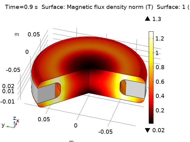
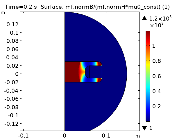
Let’s investigate the time-dependent magnetic field of a copper multiturn coil excited by a sinusoidal current using the Magnetic Fields interface with quadratic elements. The copper coil is surrounded by air and suspended by a soft iron piece, which has a nonlinear constitutive relationship (a nonlinear B-H curve).
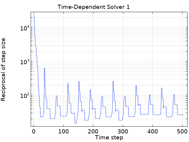
With the Times list for the Time-dependent solver set to range(0,0.1,10) and the default solver settings (Fully Coupled, Constant (Newton), Direct, and Minimal Jacobian update) and a sinusoidal coil excitation of 10 A, we find that the solution spanning 5 periods (end time 10 s) is achieved in about 100 time steps. It is important to note that the default time-stepping scheme for this kind of physics is using the Intermediate setting for Steps taken by solver. As a consequence, the specified output times put an upper limit of 0.1 s to the time step. This can be seen by inspecting the solver log. If the excitation is increased to 30 A, the upper time step constraint by means of the output times needs to be lowered (to 0.05 s, for example, with about 200 time steps in total); otherwise there is no converged solution.
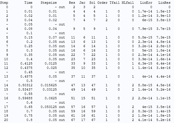
Let’s investigate the time-stepping behavior in more detail for a coil excitation of 40 A. The strategy to lower the maximum step constraint by means of the output times does not seem to be productive (even the step constraint, 0.001 s, is not working). For Times equal to range(0,0.05,10), we find a couple of failures for NLfail and the solver does actually give up with an error message after 109 time steps:
…
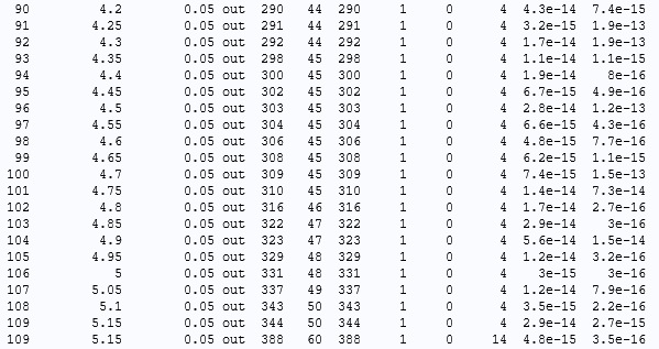
Solver log for excitation 40 A and default settings with output interval 0.05 s for the Magnetic Field of a Multiturn Coil model.
The reason for the failure can be found on the last line: 10 repeated NLfail. After 10 failures, the solver gives up before taking the next step. At this point, it has reduced the time step with a factor of 1/4 ten times. This corresponds to a 1,000,000-times smaller time step. The step size is likely not the problem here. For each try, the nonlinear solver does not converge within the maximum number of iterations.
We are simulating five full periods of the coil current, 10 s. Since the vector potential is zero for zero coil current, we need to think a bit about the scales. We can inspect the log and see that the magnetic vector potential has been given the automatic scale of “1”. By plotting the vector potential at the time where the solver stops, which is not at a zero crossing for the current, we can estimate the scale for the magnetic vector potential to around 1e-2 Wb/m. Since the default for automatic scaling is to update the absolute tolerance based on the norm of the solution, it is a good idea to change to a manual scaling of the vector potential.
Strategy for Changing the Solver Settings
Let us follow the suggested procedure under Scenario 2 above.
- Change to Manual Scaling for the magnetic vector potential, to 1e-2. By trying again, no improvement.
- Change Maximum number of iterations for the Fully Coupled solver to 10. By trying again, no improvement. This seems to be a rather nonlinear problem.
- Change Jacobian update strategy to Once per time-step. By trying again, we find that the solution is achieved in about 200 time steps with no failures reported for
NLfail(but we still cannot relax the time step constraint). - Change Jacobian update strategy to On every iteration. By trying again, we see that this really makes a difference! We can now solve even with
Freetime stepping in 28 time steps (with a slightly larger error, but with the error estimate still fulfilling the prescribed tolerances). - Next, we need to ask ourselves if the result with Intermediate time stepping and maximum step 0.05 s is an accurate result. The vector potential is computed to around 1e-2 Wb/m, except at the zero crossings (at multiples of t = 0.5 s), where it is around 1e-16 Wb/m. The scaling seems to be correct. Make a copy of the solution for reference and make a new computation with tighter tolerances.
- Make a convergence check by changing the Relative tolerance on the study to 0.0001. Notice that this also corresponds to tightening the absolute tolerance. By solving the problem for 100-times-smaller tolerances, we make a tough and good robustness test of the model. It takes around 200 time steps again and about 5% more algebraic iterations. There are no failures for
NLfailand noTfail. The nominal difference between this computed result and the copy is in the order of 1e-5 Wb/m, so we can conclude that the temporal discretization has small errors. The spatial errors are not considered in this blog post. - For an excitation of 100 A, the solution with the adjusted solver settings and with maximum time step of 0.05 s still yields a result with less than 1% error for Intermediate time stepping and the default tolerance.
In this experiment, we have found that the default solver settings are perfectly fine for the 10-A excitation. If the excitation is turned on, the nonlinear effects are much stronger. For the solver, it is a tradeoff between low costs and robustness. In the more nonlinear regime, we have to increase the robustness manually. On the other hand, the more robust settings would give a performance penalty in the case of lower excitation.
Scenario 3: Tfail Is Greater than Zero
From the solver log, we find that Tfail > 0.
A failure of a time step taken by the time-dependent solver means that the error bound with respect to the tolerances is not met, and the time step needs to be repeated with a smaller step size. The new step size is determined by means of the previously outlined mechanism. For each failure, the Tfail column is incremented. This should be seen as a failure of the time step controller, since it does not predict the local error change correctly.
The reduction of the time step and recomputation of the step are emergency operations. If this happens due to a transient in the solution that was not easy to foresee (due to its very transient nature), then this can be difficult to improve (without adding more control to the steps taken). On the other hand, if this happens regularly and without any solution transients, then there is room for improvement.
One common cause is that the error estimate is not smooth, so that it varies a lot from step to step. This is manifested by a low order used (with the BDF solver). Sometimes, reducing the Relative tolerance, or reducing the algebraic Tolerance factor to suppress algebraic errors, is the remedy. When solving PDE problems, the cause can also be that the spatial mesh is too coarse. The remedy can be to refine the mesh or introduce more spatial stabilization. A last resort for this scenario is to use Manual time stepping instead (for which Tfail is not possible, but there is also no error control). Further options include using a smaller Initial step or applying a Maximum step constraint in the Time Stepping section.
Both NLfail and Tfail could also increase. The errors of the algebraic solver could be connected to failures of the time step selection mechanism. In such scenarios, both the algebraic solver and the time-stepping mechanism should be tuned. However, this strategy can only be successful if the problem is well posed, else all bets are off.
Example: Fluid Damper
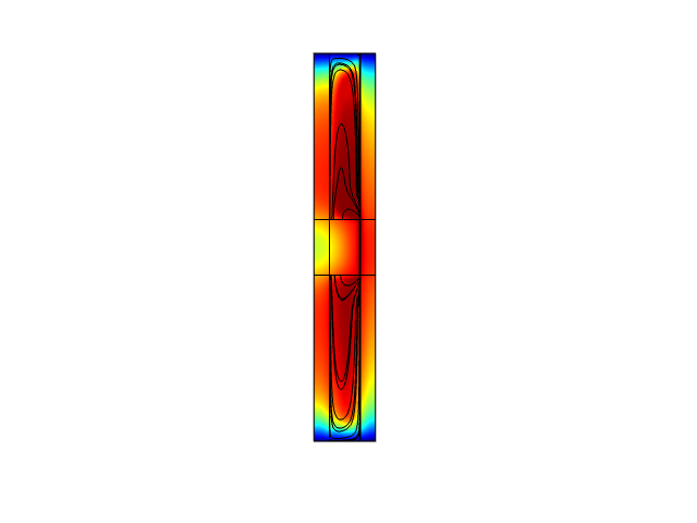
The Fluid Damper example models a device for shock isolation or suppressing earthquake-induced shaking and wind-induced vibrations. This model simulates the phenomenon of viscous heating in the device.
The model is a good example of how the time step varies in the course of a simulation. With the default solver settings, a couple of failures are recorded for Tfail.
Let us see how we can prevent these failures and how we can improve the performance of the simulation. Due to the periodic load, the fluid moves up and down interchangeably. This means that the velocity and pressure gradient fields will change directions and go through a zero-crossing (all DOFs during a short period in time). In this case, the automatic updates of the absolute tolerances can lead to complications, because the absolute tolerance will get very small values near the turning points. By inspecting the log and comparing it with the periodic piston displacement, it turns out that the Tfail happens near these points. On the other hand, the scales vary a lot.
The first idea is to turn off the Update scaled absolute tolerance check box on the time-dependent solver in the Absolute Tolerance section. This does not work. Note that in the Algebraic variable settings section, the Error estimation is set to Exclude Algebraic and the Tolerance factor for Pressure (comp1.p) is set to 0.05.
Let’s try to use manual scales on the variable nodes under the Dependent Variables node. Set Method in the Scaling section to Manual and use the Scale 1e7 for the Pressure, 1e2 for the Temperature, and 1e1 for the Velocity field. In addition, use a Tolerance factor of 0.1 for the pressure and the temperature, and 0.5 for the velocity. There are no more Tfail, but instead, there are 6 NLfail. The main benefit is that only around 400 time steps are used instead of 1300. The NLfail can be reduced by setting the Maximum number of iterations on the Segregated node to 15 and setting the Dimension of iteration space for the Anderson acceleration to 8, for example. These changes save a lot of computational time.
Example: Inductor in an Amplifier Circuit
The Inductor in Amplifier Circuit example illustrates how to combine an electric circuit simulation with a finite element simulation. In the context of this blog post, it is an example of adjusting the Tolerance factor to optimize the behavior of the time-stepping scheme. In this case, extra algebraic steps with the Minimal setting for the Jacobian update are sufficient to save work. With the solver settings as stored in the model, we find that the solution for the stationary and time-dependent Study 2 is within 170 steps, 10 TFail, and 1 NLfail.
By lowering the Tolerance Factor to 0.1 and increasing the Maximum number of iterations to 6, we find that the number of steps is reduced to 127 with 2 TFail and 0 Nfail without touching the settings for the Jacobian update. The remaining Tfail originate from the initial step. They can also be avoided by, for example, lowering the initial step to 1e-9s. However, the benefit from this is marginal. For this example, tighter tolerance also leads to a significantly more efficient solution process.
Concluding Thoughts on Automatic Time Steps and Order Selection
In this blog post, we have presented strategies on which “knobs to turn” in the solver settings and what to read from the time-dependent solver log. Further information on these topics can be found in COMSOL’s Knowledge Base.
Related Resources
Learn more in these articles from the COMSOL Knowledge Base:




Comments (0)