Thermal Equilibrium and Nonequilibrium Heat Transfer in Porous Media

Porous materials have a growing range of applications thanks to their availability, cost, and special thermal properties. For example, foam materials are increasingly used in different aeronautical applications due to their excellent mechanical and thermal properties. Porous structures are also found in the batteries used in electric vehicles. We even find countless porous materials in nature, such as soils, rocks, and wood; and we take advantage of their thermal properties when we make use of them. The many industrial applications of porous materials require them to have optimized thermal performance.

Heat Transfer on the Microscopic Scale

Let’s take a closer look at the heat transport in a porous structure on the microscopic level. As discussed in our previous blog post, we use these findings to verify and understand the flow equations at the macroscopic level. In that example, the flow is isothermal, so we do not investigate the implication of the pore geometry in the heat transport. Since the thermal properties of fluids might significantly differ from the properties of solids, the interaction of these is essential for understanding how heat transport in porous media works.

Temperature evolution of a cooled porous structure. The initial local nonequilibrium reaches thermal equilibrium over time.

Let’s use the same example as shown in the previous blog post, and inject a fluid that is much warmer than the porous matrix. We observe that the temperatures of the porous matrix T_\textrm{s} and fluid T_\textrm{f} initially differ, and balance gradually over time. Of course, this depends on the boundary conditions and thermal properties of the fluid and solid. In many applications, the assumption T_\textrm{s}=T_\textrm{f} is valid and we speak of (local) thermal equilibrium, whereas in other applications, T_\textrm{s}\neq T_\textrm{f} applies and we speak of (local) thermal nonequilibrium. The addition “local” refers to the pointwise comparison of the temperatures T_\textrm{f} and T_\textrm{s}.

Heat Transfer Under Thermal Equilibrium

We only need one equation to describe the average temperature of the whole (solid and fluid) porous structure under the local thermal equilibrium assumption. Based on the conservation of energy and by applying mixing rules, the following equation is obtained for the heat transport equation

(1)

It is no surprise that this is very similar to the well-known heat transfer equation. The thermal properties of the fluid and porous matrix are combined as effective properties, which are the effective volumetric heat capacity and effective thermal conductivity

The indices \textrm{f} and \textrm{s} stand for the fluid and solid, respectively, and \rho is the density, C_p the heat capacity at constant pressure, and \theta_\textrm{s} is the solid volume fraction. We assume a fully saturated porous medium, so the porosity would correspond to the fluid volume fraction, \theta_\textrm{f} =1-\theta_\textrm{s}.

For thermal conduction, the effective thermal conductivity k_\textrm{eff} depends on the structure of the porous medium as well as on the thermal conductivity of the solid and fluid. Three options to calculate the effective thermal conductivity k_\textrm{eff} are available in the software:

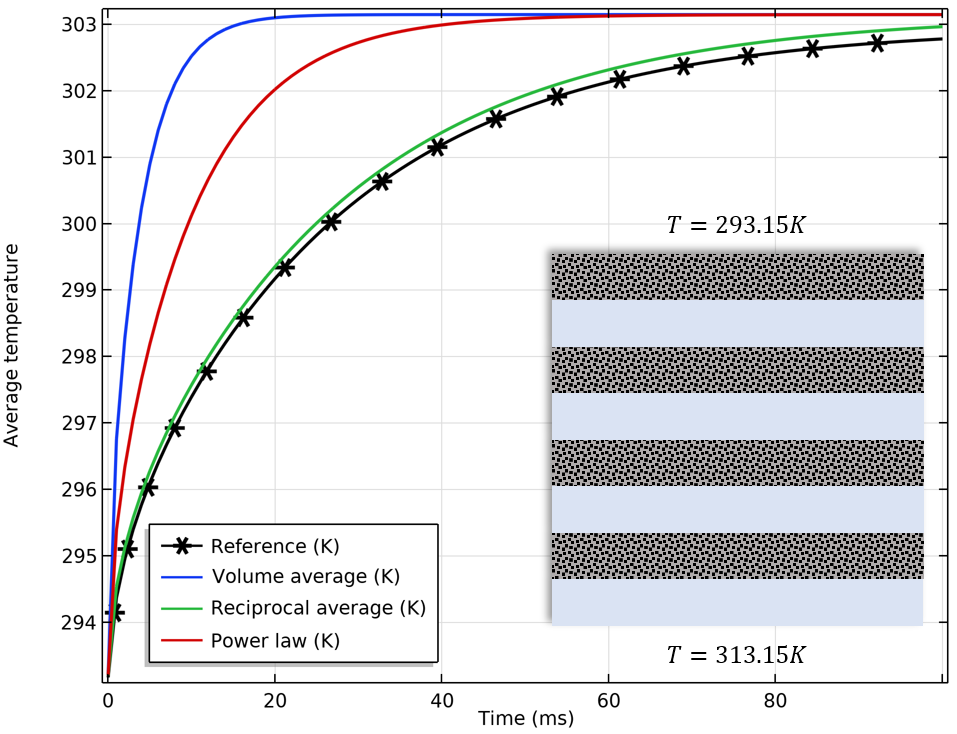
1. Volume average, which symbolically represents solid and fluid stripes in parallel to the heat flux, with k_\textrm{eff}=\theta_\textrm{s} k_\textrm{s} + \theta_\textrm{f} k_\textrm{f}
2. Reciprocal average, for solid and fluid stripes perpendicular to the heat flux, with \frac{1}{k_\textrm{eff}}=\frac{\theta_\textrm{s}}{k_\textrm{s}} + \frac{ \theta_\textrm{f}}{k_\textrm{f}}
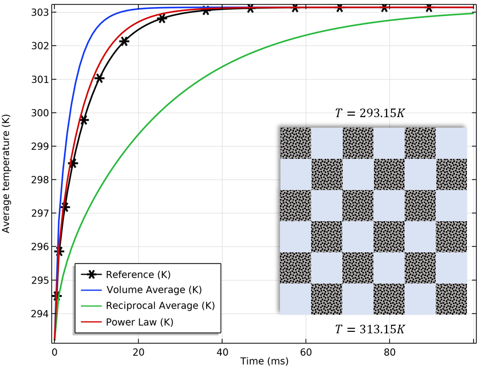
3. Power law, for a random geometry with similar thermal conductivities for the solid and fluid, with k_\textrm{eff}=k_\textrm{s}^{\theta_\textrm{p} }\cdot k_\textrm{f}^{\theta_\textrm{f}}

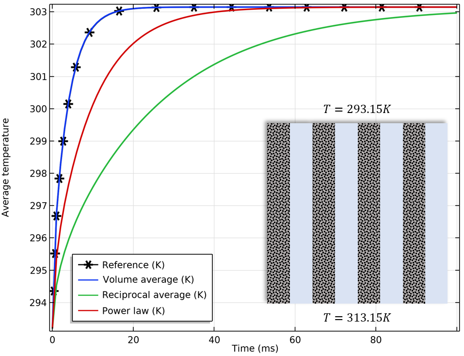
We illustrate these three averaging techniques by using an artificial example of a porous material, and compare the results for the different options with those of the calculated value.

Comparison of the average temperature for different effective thermal conductivity options. From left to right: Solid (gray) and fluid (blue) materials arranged in parallel, in series, and in a check pattern. The heat flux is produced by a prescribed temperature difference between the upper and lower boundaries.

The finer the structure, the better the approximation for the reciprocal average and power law. The true effective thermal conductivity ranges between the volume average and the reciprocal average, which are the upper and lower bounds according to the rule of mixtures. If convection is the dominant effect, the effect of the mixing rule for the thermal conductivity is less important.

A porous material can also consist of several solids and immobile fluids; e.g., a rock consisting of different minerals or trapped fluids. This can also be considered in the model, and the effective material properties are then calculated accordingly. For example, the volume average thermal conductivity of the porous matrix consisting of i different materials is calculated according to k_\textrm{s}=\displaystyle\sum_{i=1}\theta_{\textrm{p}i}k_{\textrm{s}i}.

Thermal Dispersion

Thermal dispersion is another important effect related to the porous microstructure. Typically, for convection-dominated regimes, the fluid follows a swirled path at the pore scale, which enhances the heat exchange between solid and fluid phases. This is macroscopically described by an additional thermal conductivity contribution to the heat transfer equation (Eq. 1), k_\textrm{disp}=\rho_\textrm{f} C_{p,\textrm{f}} D_{ij}, where D_{ij} is the dispersion tensor due to the fast velocity field.

We compare the results of the average temperature for the example shown in the previous blog post. The graph below shows the average temperature computed from the microscale approach, and the values obtained from the averaged macroscopic equations with and without thermal dispersion.

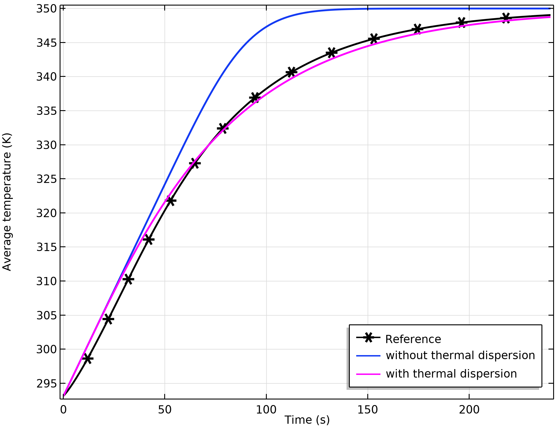
Comparison of the average temperature for the microscopic and macroscopic approaches. There is a better match when thermal dispersion is included.

Heat Transfer Under Local Thermal Nonequilibrium

As stated at the beginning of this blog post, local thermal equilibrium is not always attained. In particular, the difference between solid and fluid temperatures can be substantial for fast nonisothermal flows, short time scales, or when strong dependencies on additional effects (for instance, phase transitions) occur. Then, Eq. 1 is not sufficient, the energy balance for each phase must be considered separately, and the heat exchange between the two phases must be accounted for in an explicit way. This is accomplished with a two-temperature model. The Local Thermal Nonequilibrium approach (Ref. 1) solves for two temperature fields, and couple these through a heat source/sink:

The heat exchange between the solid and fluid is considered by the term on the right-hand side, where q_\textrm{sf} (W/(m³ K)) is the interstitial heat transfer coefficient that depends on the thermal properties of the phases as well as on the structure of the porous medium; more precisely, the specific surface area of contact.

An excellent example where nonequilibrium heat transfer is present is a thermal energy storage (TES) unit. This device works as follows: Water is heated up by a solar collector, and it circulates through a tank containing paraffin-filled capsules. During the charging period, the paraffin inside the capsules is heated above its melting temperature. As a result, the solar energy is stored in the form of sensible and latent heat, which allows more energy storage over longer periods.

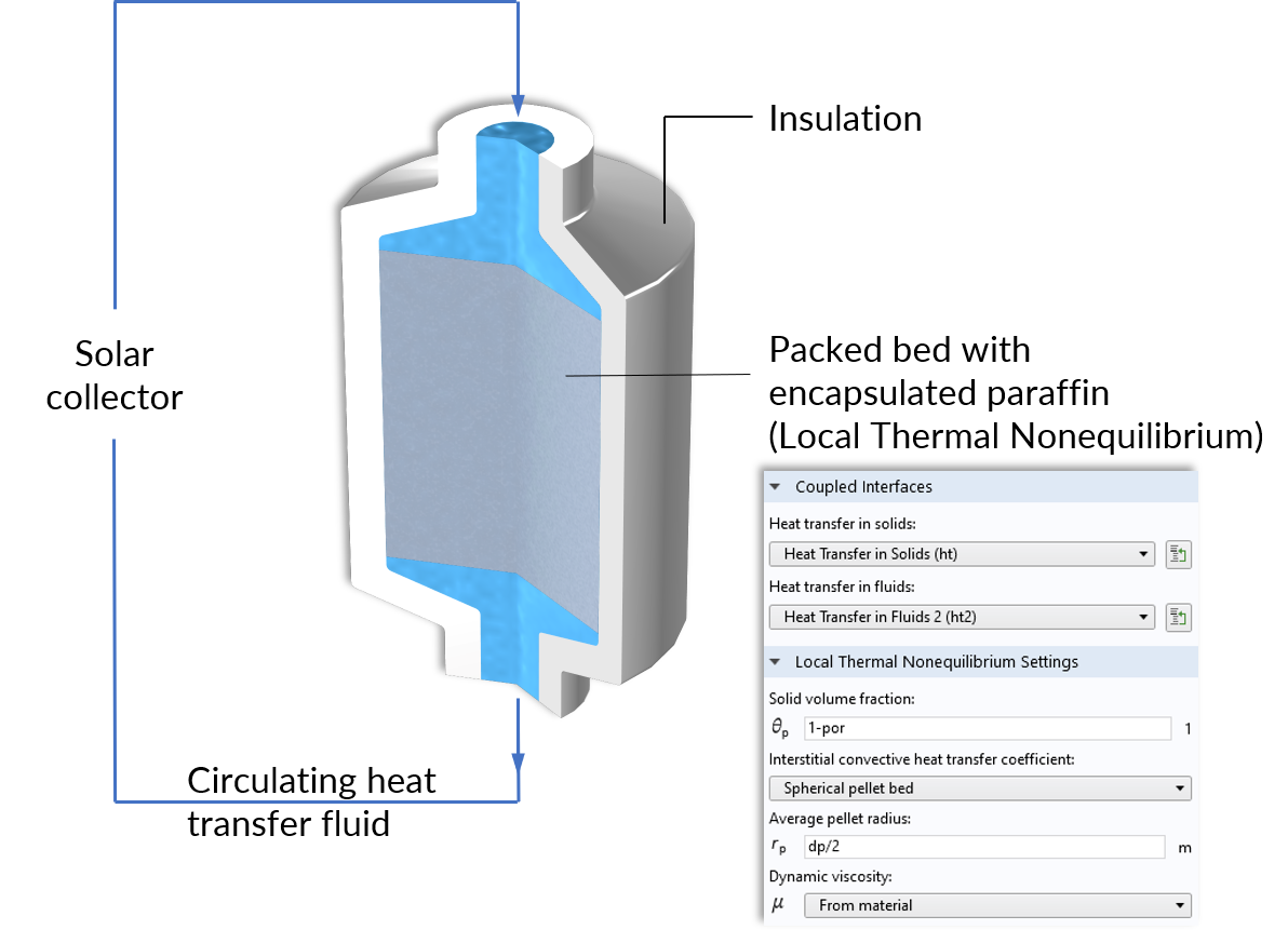
Operating principle of the thermal storage unit and the Local Thermal Nonequilibrium multiphysics coupling node for the packed bed.

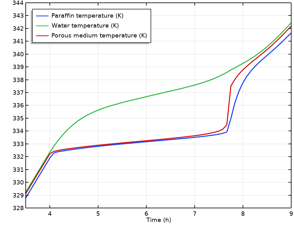
Paraffin, water, and average temperature in the tank during the charging period.

The encapsulated paraffin takes a longer time to heat up as compared to water, so the time until the tank is fully charged cannot be estimated by the water temperature alone. The Local Thermal Nonequilibrium multiphysics interface provides the means to couple the heat transfer in water and paraffin.

Final Remarks on Modeling Heat Transfer in Porous Media

We have taken a closer look at the mechanism of heat transfer in porous media at microscopic and macroscopic levels. The macroscopic equations with effective thermal properties provide a very good approximation for modeling homogenized heat transfer in porous media. Complex calculations of pore-scale flow can also be included in the COMSOL Multiphysics® software. For example, you can compute heat transfer equations for the simulation of representative elementary volumes (REV) in order to obtain averaged values for large-scale, real-life applications.

Reference

1. D. A. Nield and A. Bejan, Convection in Porous Media, 4^th ed. Springer, 2013.

Try It Yourself

Try the packed bed latent heat storage model featured in this blog post by clicking the button below. Doing so will take you to the Application Gallery, where you can download the MPH-file.