Using Curvilinear Coordinates

Curvilinear coordinates are a coordinate system where the coordinate lines may be curved. The new user interface for automatic computation of curvilinear coordinates is a very practical addition to version 4.3b for those working with anisotropic materials in free-form CAD designs. If you have a generic bent shape and try to apply the usual coordinate systems like Cartesian, cylindrical, or spherical, you are out of luck. Curvilinear coordinates are needed to smoothly follow the design, which typically has no mathematical “closed form” representation.

The Curvilinear Coordinates Interface

The new user interface makes computing such a coordinate system easy by solving a flow-like equation (or in some cases an elasticity equation) where you simply define an inlet and an outlet for the “flow” of your coordinate’s principal axis. Now, curvilinear coordinates that follow curved geometry objects aren’t necessarily uniquely defined. What happens for example if the cross section of your model has narrow parts? Is the anisotropic material of the model trimmed as if by a cookie cutter or is it squeezed together in the narrow parts? Does your object have sharp corners? Because of these ambiguities, three different methods are offered: Diffusion Method, Elasticity Method, and Flow Method. These all give slightly different coordinates corresponding to the underlying equation solved (the equations are outlined in the COMSOL Multiphysics Reference Manual). There is actually also a fourth method, User Defined, where you are free to type in your own mathematical expressions for the curvilinear coordinates’ principal vector field.

The curvilinear coordinates can be used not only for defining anisotropic materials, but for all kinds of other applications, such as electrical currents or visualization. In a new tutorial model of the Nonlinear Structural Materials Module, four different curvilinear coordinates interfaces are used to visualize the fiber directions of an anisotropic Holzapfel-Gasser-Ogden material model. This is a hyperelastic material model for biomechanics applications and is useful for representing collagenous soft tissue in arterial walls.

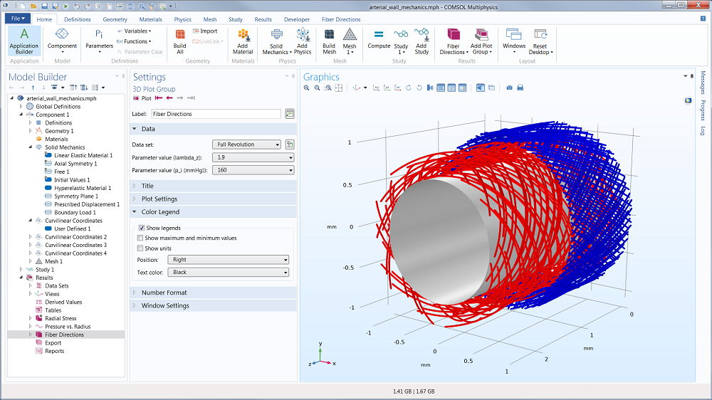
The figure shows the fiber orientation for different fiber families in the media and adventitia. Arteries have layered structures with the intima inside, followed by the media and the adventitia. The two outer layers are predominantly responsible for the mechanical behavior. Both layers are made of collagenous soft tissues that show prominent strain stiffening. Families of collagen fibers give each layer anisotropic properties. These fiber reinforced structures enable blood vessels to sustain large elastic deformation. The Holzapfel-Gasser-Ogden (HGO) constitutive model described in a literature reference captures the anisotropic nonlinear mechanical response observed in excised artery experiments. This model demonstrates how this hyperelastic material is used in COMSOL Multiphysics, and the results are compared to those reported in the literature. The anisotropic directions are visualized using the new curvilinear coordinates user interface.

An S-Shaped Heat Transfer Example

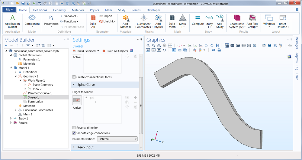
Let’s now take a look at a very simple heat transfer example and how we can use the new tool to compute for the temperature in an S-shaped geometry with an anisotropic material that follows the shape. Similar structures are found in smartphones and flat screens and are used as passive heat sinks where a highly anisotropic thermal conductivity spreads heat laterally. This particular example is created in COMSOL by using the Sweep geometry operation to sweep a rectangular cross section along an S-shaped curve.

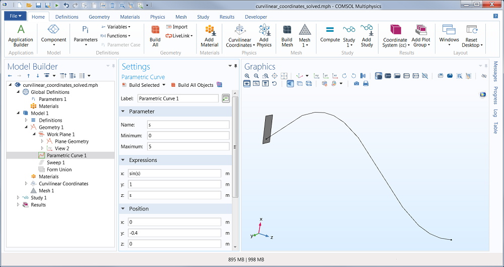
A rectangular cross section and a parametric curve used as a basis for a geometric sweep.

The final swept geometry.

We can, of course, also import a CAD file. Once we have created the geometry, we continue by adding a Curvilinear Coordinates user interface from the Mathematics branch of the Model Wizard. The next step is to define an Inlet and an Outlet boundary condition. This will define the principal direction of the coordinate system.

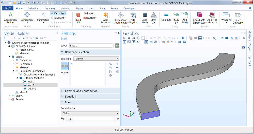
An Inlet boundary condition is used to define the source of the curvilinear coordinates’ principal direction.

The other directions are computed automatically but you can guide the definition of those directions by, for example, aligning it with one of the coordinate axes. In this example we use the Diffusion method. Also, if we would like an orthogonal coordinate system to be automatically defined, then we can select the “Create base vector” check-box, as seen in this screenshot:

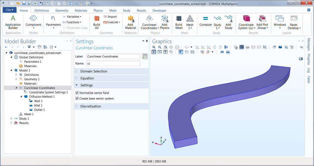
The “Create base vector” check-box.

Now we can just solve and get a visualization of the coordinate system:

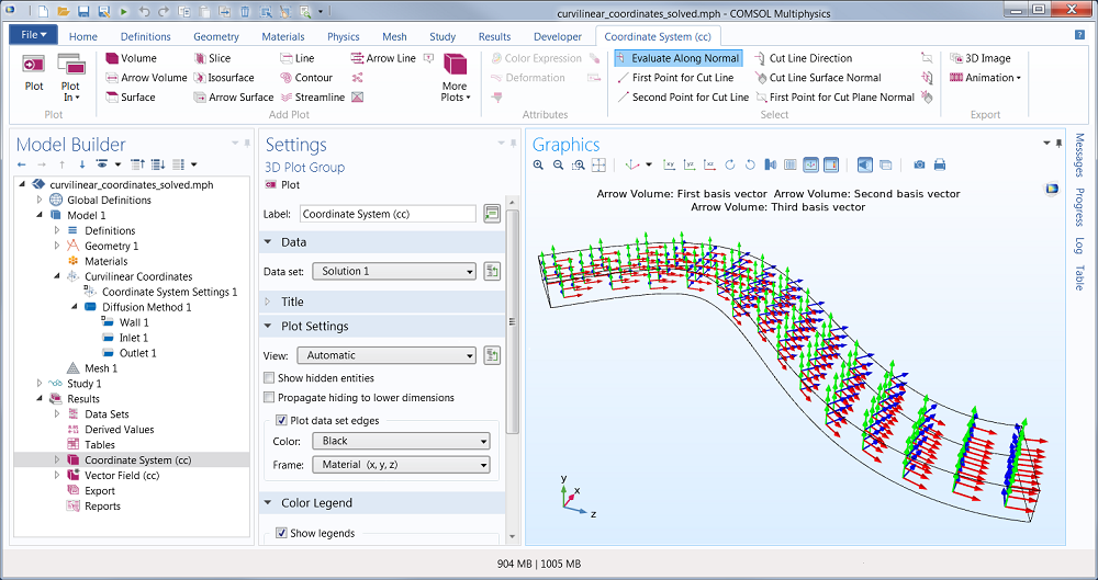
A visualization of the computed curvilinear coordinates.

In this example we also add a Heat Transfer in Solids user interface, and to get something interesting we create a disk (using a Work Plane and a Circle) at the top surface on which we defined a low temperature condition. At the same time, we assign a hot temperature condition along the entire bottom surface of the model. When using an anisotropic material with a high conductivity in one direction, this is the temperature profile we get:

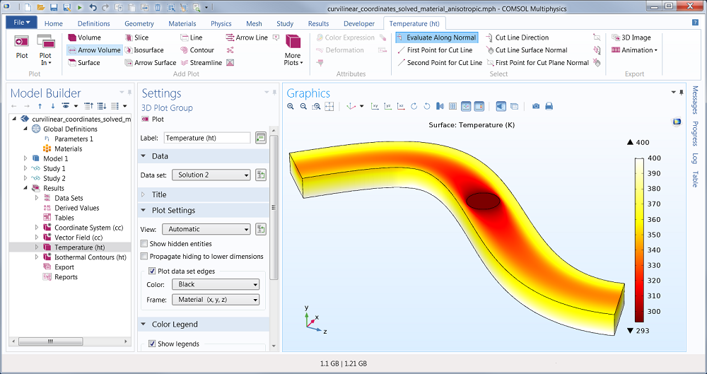
Temperature field in an anisotropic material.

We can see that the heat is spreading in the length-direction of the shape.

Anisotropic Material

You may ask: How do I create and reference an anisotropic material? The first step is to create the material under the Materials node in the Model Tree. In this case, the thermal conductivity in the local x-direction is high, while it is low in the local y- and z-directions. We can formally write this as: k_x >> (k_y=k_z).

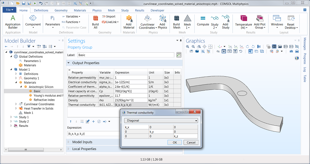
Definition of an anisotropic thermal conductivity.

But this is just the definition in a local (abstract) coordinate system. Then we need to reference the curvilinear coordinates that were automatically computed. This is done in the Heat Transfer in Solids settings window:

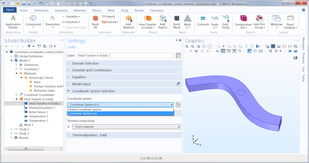
Reference to the computed curvilinear coordinates.

By referencing the Curvilinear System in this way, the anisotropic thermal conductivity defined by k_x, k_y, and k_z above will “know how to bend” accordingly.

Study Settings

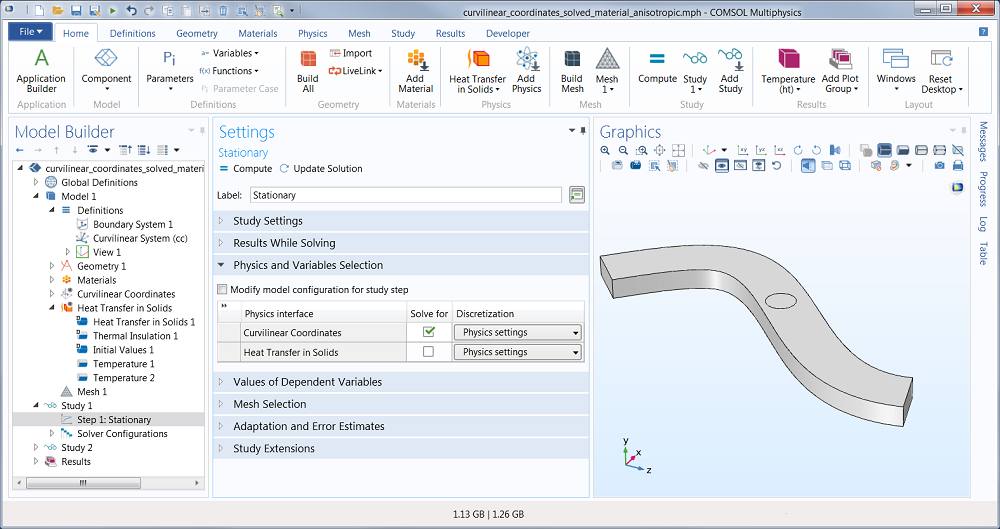
Finally, we need to make sure that we first solve for the curvilinear coordinates and then for the heat transfer in solids. (Otherwise the heat transfer in solids wouldn’t know what material to use.)

This is done by using two Studies. Study 1 is used to compute the curvilinear coordinates and Study 2 is used for the heat transfer in solids. These are the settings for Study 1:

The Study 1 settings.

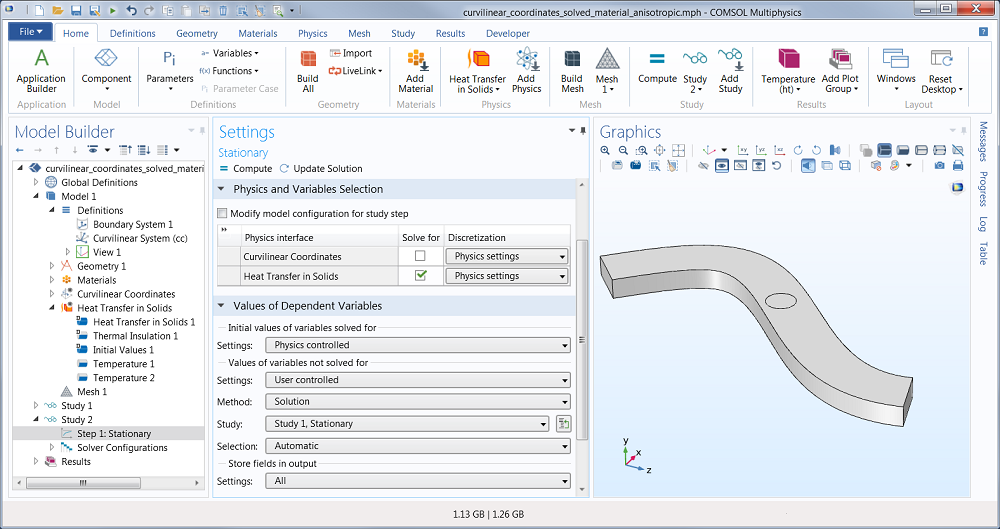
The Study 2 settings are similar, but here we also need to define what to do with values of variables not solved for. This is the solution of Study 1 and we just reference that in the section called values of dependent variables:

The Study 2 Settings.

Now solve for Study 1 first and then Study 2. That’s it. We’ve seen how quickly we can set up a custom coordinate system for any shape. In this example we used a simple S-shaped geometry, but you can also try this now for geometry models with branches and other more complex geometrical features. Since this curvilinear coordinate method is computational, it works for any CAD model. Enjoy!