Using Data Filtering to Improve Model Performance

Have you ever been in the situation where you want to use some experimental data as a load or boundary condition? If this data varies over space or time and is noisy, you might need a very fine mesh, or the solver might need very short time steps. Practically speaking, we often don’t want or need this. One possible solution is to filter the input data to make it smoother. Let’s find out more!

Filtering Noisy Data with Equation-Based Modeling

We will start by considering some sample input data, as shown in the figure below. For now, let’s not concern ourselves with what the data represents, and imagine that the horizontal axis could represent either space or time. We can observe that the data has some significant noise, as well as apparent trends. We would like to reduce this noise before using this data in our model.

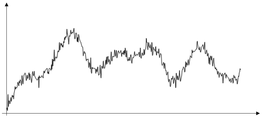
Sample of data with significant noise.

What we can do here is use a so-called Helmholtz filter. This type of filter was recently proposed and proved quite useful in the area of topology optimization. In fact, this functionality is a built-in feature of the Optimization Module, but it can also be manually implemented, which is what we will do here.

The Helmholtz filter simply solves the governing partial differential equation:

where D is the input data and u is the filtered data.

There is one parameter to this equation, R, which we will call the filter radius.

Along with the governing equation, we need boundary conditions. For reasons discussed below, we will start with the homogeneous Neumann condition, meaning that the gradient of the fields at the boundaries is zero. To solve this equation along with this boundary condition, we will use equation-based modeling via the Coefficient Form PDE interface in a 1D Component.

To get started, let’s read our experimental data into an Interpolation table feature, as shown in the screenshot below. Note that the Extrapolation is set to Constant. As we will see shortly, due to the boundary conditions in our Helmholtz filter, we need to have some data for the buffer region of space or time outside of our range of interest.

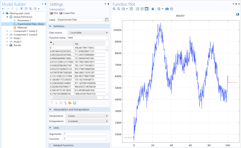
Reading in the experimental data and setting the Extrapolation method.

Next, let’s introduce a 1D Component into our model and set the Unit system to None.

Then, create an Interval feature into the Geometry, as shown in the screenshot below. Note the additional regions on the sides of the data range of interest.

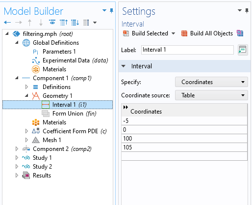
Defining the domain over which the filter is applied.

Now we introduce a Coefficient Form PDE interface into the Component, in terms of a single unknown, u, as shown in the screenshot below. We will leave the Discretization at the default Lagrange Quadratic. Again, let’s keep everything dimensionless.

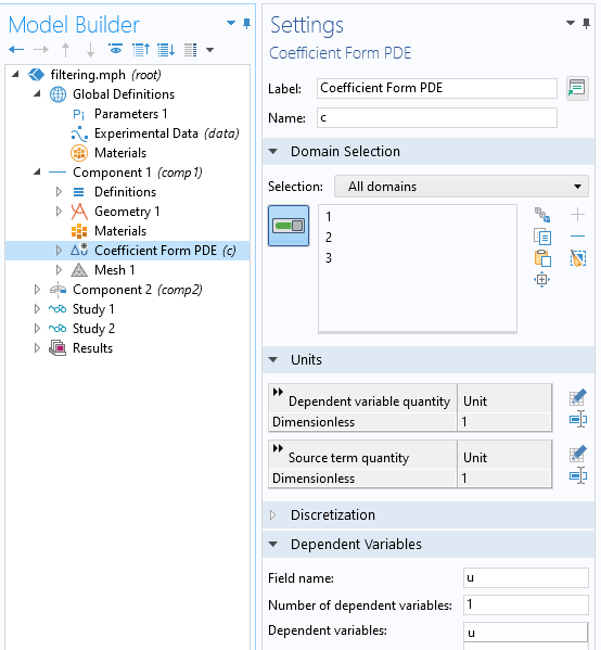
Within the settings for the Coefficient Form PDE feature, we define the settings as shown below. The Diffusion Coefficient is set to the square of the global parameter FilterSize, and the Absorption Coefficient is 1. The source is our experimental data, and all other terms are set to zero.

The default boundary condition of Zero Flux is the desired homogeneous Neumann condition, and we will fix the derivative of our filtered data set to be zero at the ends of the computational domain. This does introduce an end effect to the filter, which is why we introduced the additional padding region to the geometry, and to the data.

We could alternatively use the Dirichlet boundary condition, which would fix the value of u at the boundary. We also need to manually set the mesh size to be smaller than the resolution of our experimental data.

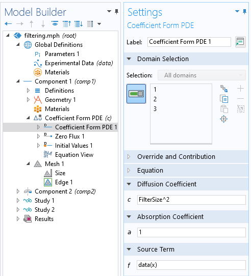
Using equation-based modeling to define the Helmholtz filter equation.

Using the Helmholtz Filter Equation for Model Data

We can now solve for different values of the filter size and compare results. As we see below, a very small filter size has almost no effect. Larger filter sizes lead to more smoothing, and as the filter radius gets large, the filtered data approaches the average of the original.

It is important to realize this key property of the Helmholtz filter: It is energy preserving as long as the homogeneous Neumann boundary conditions are used. This means that the integral of the original data and the filtered data over the entire computational domain will be the same.

Note that this is not precisely true over the subdomain without the buffer zones at either end. It is also important to note that the Dirichlet boundary condition is not energy preserving and should thus be used with caution.

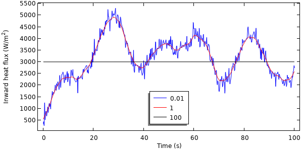
Examples of filtered data with various filter radii.

Now that we have filtered the data, let’s use it in a model. We will consider the transient heating of a 2D axisymmetric piece of material, and the filtered data will represent the applied heat load on the exposed surfaces. Since our thermal model is going to be in a different component within our model, we need to introduce a way to move our data from our 1D component into the time dimension for use within a 2D axisymmetric component. This is done via the General Extrusion operator, where we define a Destination Map for the x-expression of t. This feature will map, or extrude, the data from the 1D component onto the time axis, and make it generally available everywhere within the model.

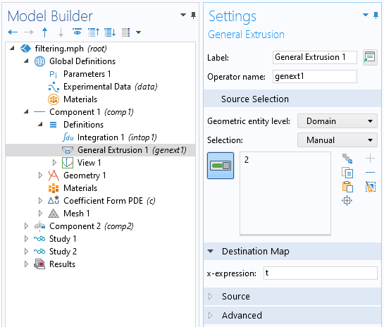
Screenshot showing the settings within the General Extrusion operator.

Within the thermal model in the 2D axisymmetric component, we can apply a heat source, as shown in the screenshot below, where the heat load is comp1.genext1(u)[W/m^2]. Note that we add units to this, as u is dimensionless.

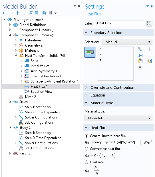
Calling the filtered data defined in Component 1 from the thermal model in Component 2.

We can modify our study to contain two steps. The first step is a Stationary step, solving for the filtering equation, and the second is a Time Dependent step, solving the thermal problem. We will solve to a tighter relative tolerance of 1e-4 and output the results at all time steps taken by the solver, as described in this Knowledge Base entry.

As an aside, it is also worth noting that if the data instead had distinct, sharp changes in magnitude without noise, you should instead use the Events interface to inform the solver.

Solving for different values of filter radius, and plotting peak temperature within the domain over time, we can see the effect of the filtering on the thermal solution. We see that for this case, there’s only a very small effect on the peak temperature over time.

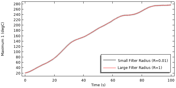
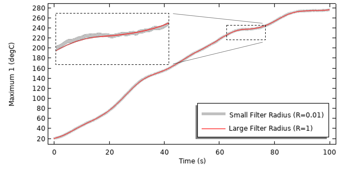
Results of the thermal model, solved with different filtering applied to the transient heat load.

The dramatic difference here is in the solution time. Solving for a model without filtering takes about 700 adaptive time steps in all, while solving the model with a moderate filter size takes about 130 time steps, leading to over a five-fold improvement in solution time!

Concluding Thoughts

Here, we have shown how an additional component and equation can be used to implement a Helmholz filter on data that we want to input into our model. We can do this not only with 1D data, but also with 2D or 3D data, and we can implement this filter over any arbitrary geometric shape and with any arbitrary density of input data. In 2D and 3D especially, this method will outperform most other filtering techniques, because it takes advantage of the local compact support of the finite element basis functions and permits a nonuniform spatial mesh discretization. This thereby results in sparse linear matrices that can be solved very efficiently.

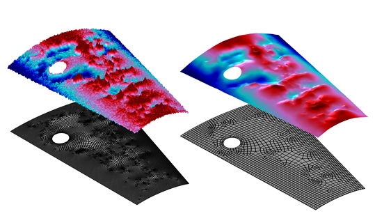
Spatial filtering via a Helmholtz filter on an arbitrary surface. The filtered data can be well-represented with a coarser mesh.

An example of 2D smoothing is visualized in the image above of unfiltered and filtered fields over an arbitrary surface. Note that filtering the data would allow a model that uses this data to be solved on a relatively coarser mesh, giving us an additional computational benefit. It turns out that we can even use this Helmholtz filter to design a mesh that conforms well to the variations in our input data, but that is a topic for another day!

Try It Yourself

The files associated with these approaches are available for download here: