
Today, we compare the Boussinesq approximation to the full Navier-Stokes equations for a natural convection problem. We also show you how to implement the Boussinesq approximation in COMSOL Multiphysics software and discuss potential benefits of doing so.
Application: Natural Convection in a Square Cavity
For our example, we will use a model that couples the Navier-Stokes equations and the heat transfer equations to model natural convection in a square cavity with a heated wall. The temperature on the left and right walls is 293 K and 294 K, respectively. The top and bottom walls are insulated. The fluid is air and the length of the side is 10 cm.
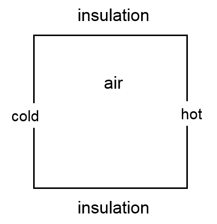
We will use this model to compare the computational cost of three different modeling approaches:
- Solving the full Navier-Stokes equations (Approach 1)
- Solving the full Navier-Stokes equations with pressure shift (Approach 2)
- Using the Boussinesq approximation with pressure shift (Approach 3)
Each of these three approaches and their variables are defined here.
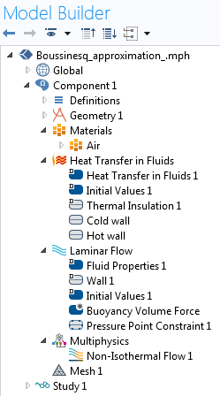
In COMSOL Multiphysics, the model is solved with a stationary study using the Laminar Flow, and Heat Transfer in Fluids interfaces, and the Non-Isothermal Flow multiphysics coupling:
While setting up the model, it is important to check whether the flow is laminar or turbulent. For a natural convection problem, this is done by calculating the Grashof number, Gr. For an ideal gas, it is defined as
The Grashof number is the ratio of buoyancy to viscous forces. A value below 10^8 indicates that the flow is laminar, while a value above 10^9 indicates that the flow is turbulent. In this case, the Grashof number is around 1.5 \times \hspace{1pt} 10^5, meaning that the flow is laminar.
Approach 1
When using the full Navier-Stokes equation, we set the buoyancy force to \rho \mathbf{g}:
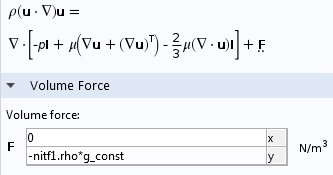
The buoyancy term is added using a volume force feature. The terms nitf1.rho and g_const represent the temperature- and pressure-dependent density, \rho, and the gravitational acceleration, \mathbf{g}, respectively.
Approach 2
When using the Navier-Stokes equations with pressure shift, we have to make three changes.
First, we need to change the definition of the volume force to (\rho-\rho_0)\mathbf{g}, as such:
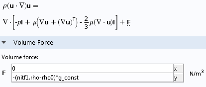
The term rho0 refers to the reference density \rho_0.
Next, we evaluate the reference density \rho_0 and the reference viscosity \mu from the material properties in a table of variables:

Here, pA and T0 represent the reference temperature and pressure.
The air viscosity is set to the constant \mu_{0}:

Approach 3
Finally, when using the Boussinesq approximation, we need to set the buoyancy force to -\rho_0\frac{T-T_0}{T_0}\,\mathbf{g}:
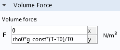
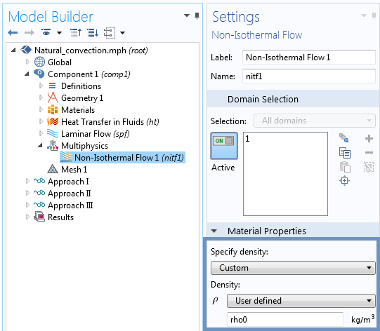
As with Approach 2, we also evaluate the reference density and viscosity from the material properties. A third and final step with Approach 3 is to set the fluid density to the constant reference density \rho_{0} (the Boussinesq approximation states that the density is constant except in the buoyancy term).
Note: If your model includes a pressure boundary condition (open domain), set the pressure to the hydrostatic pressure -rho0*g_const*y for Approach 1 or to 0[Pa] for Approach 2 and Approach 3. The boundary conditions for models including gravitational forces are also discussed here.
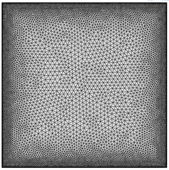
The mesh is made of 15,000 triangular elements and 1,200 boundary layer elements. These are first-order elements.
Results
The resulting velocity magnitude and streamlines are nearly identical for all three approaches. The maximum temperature difference between Approach 1 and 2 is less than 2 \times \hspace{1pt} 10^{-6} K and the maximum temperature difference between Approach 1 and 3 is around 5 \times \hspace{1pt} 10^{-4} K. The only thing that differs is the simulation time.
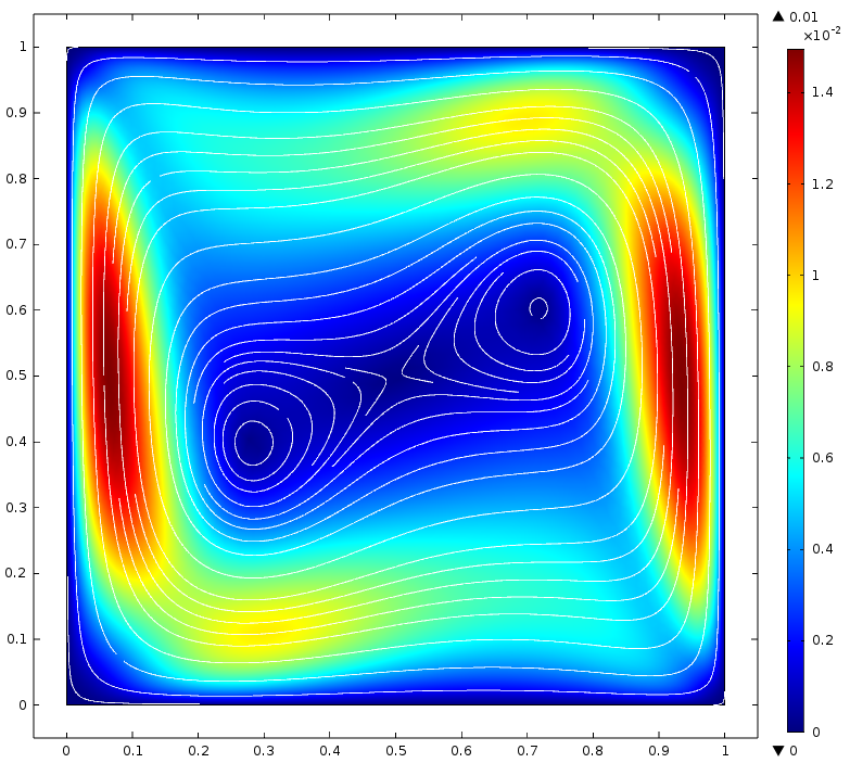
Velocity magnitude and streamlines.
Because of the short running time of this 2D simulation (around 30 seconds), we look at the computational load by comparing the number of iterations it takes the solver to converge to the steady-state solution. The number of iterations, in this case, is nearly proportional to the CPU time.
The table below compares the number of iterations across all three approaches.
| Approach 1 | Approach 2 | Approach 3 | |
|---|---|---|---|
| Number of Iterations | 39 | 55 | 55 |
These results are very surprising!
While the Boussinesq approximation is supposed to reduce the nonlinearity of the model and the number of iterations required for convergence, the full Navier-Stokes equations (39 iterations) can be solved faster than the Boussinesq approximation (55 iterations). We also note that the use of Navier-Stokes equations with a pressure shift leads to the same number of iterations as the Boussinesq approximation.
To better understand these results, we can run a second set of simulations after disabling the pseudo time-stepping algorithm. Pseudo time stepping is used for stabilizing the convergence toward steady state in transport problems. The pseudo time stepping relies on an adaptive feedback regulator that controls a Courant–Friedrichs–Lewy (CFL) number. The pseudo time stepping is often necessary to get the model to converge. In this particular case, however, it is not needed .
Here’s a look at the COMSOL Multiphysics settings window for the default solver settings with pseudo time stepping:
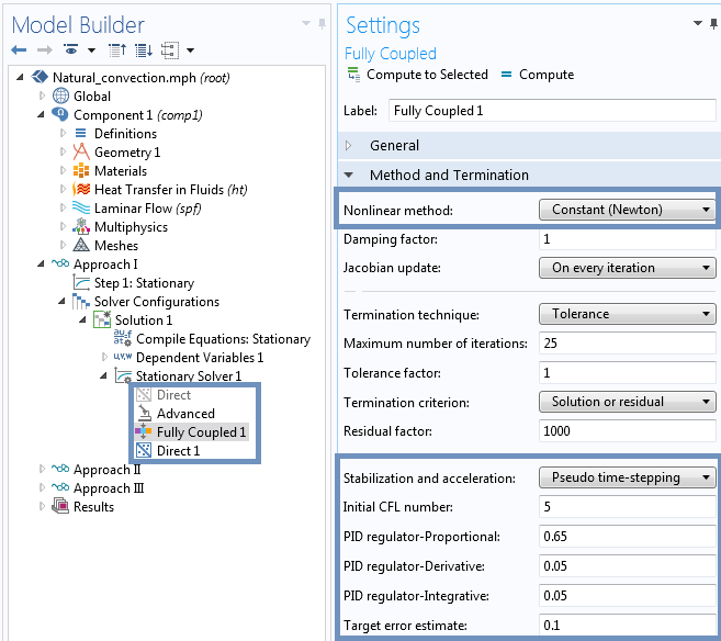
The following snapshot shows the updated solver settings without pseudo time stepping. We recommend that you always keep pseudo time stepping switched on, unless you feel comfortable tuning the solver settings.
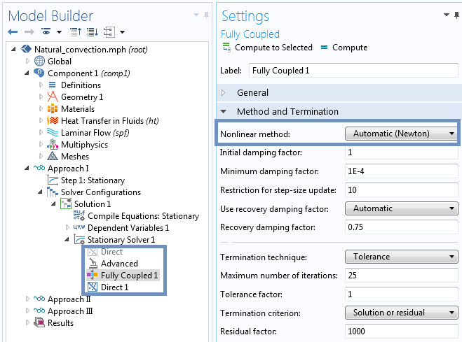
Note on the solver settings for natural convection:
Due to the very strong coupling between the laminar flow and heat transfer physics in natural convection modeling, always use a fully coupled solver. The COMSOL software automatically switches to a fully coupled solver when a volume force is added in the laminar flow physics, meaning that you are modeling natural convection.
This second table shows the number of iterations without pseudo time stepping:
| Approach 1 | Approach 2 | Approach 3 | |
|---|---|---|---|
| Number of Iterations | 9 | 7 | 7 |
These results make more sense than the previous ones with pseudo time stepping. This is because Approach 3, the most linear problem, now converges faster than Approach 1. What is surprising is that Approach 2 and Approach 3 converge with the same number of iterations.
Comparing these results with the first set of results, a speed-up of 8 (from 55 to 7 iterations) is observed for the third approach — the Boussinesq approximation. These results also indicate that the number of iterations in the first set of results not only depend on the linearity of the problem, but also on the tuning of the pseudo time-stepping algorithm.
What Did We Learn?
Here, we have discussed the implementation and benefits of the Boussinesq approximation as well as using the pressure shift method. The results show that, for this particular model, there are no real benefits in terms of computational time for using the Boussinesq approximation, regardless of whether or not pseudo time stepping is enabled. This is generally the case since the Boussinesq approximation is only valid when the nonlinearity is small. A much shorter computational time for the Boussinesq approximation with respect to the full Navier-Stokes equations would indicate that the Boussinesq approximation might not be valid.
Because of the small speed-up observed with the Boussinesq approximation and the fact it is not always easy to know a priori if the Boussinesq approximation is valid, we generally recommend solving for the full Navier-Stokes equations. Implementing the pressure shift (Approach 2 and 3), however, does avoid round-off errors and simplifies the implementation of time-dependent problems as well as models with open boundaries. This will be the object of a future blog entry.
Using Approach 3 (Boussinesq approximation with pressure shift) involves more implementation steps and does not reduce the number of iterations as compared with Approach 2 (Navier-Stokes equations with pressure shift). The final simulation time might be slightly shorter for Approach 3, since it does not require the evaluation of the temperature- and pressure-dependent density and the temperature-dependent viscosity, but this speed-up might not be noticeable.
The number of iterations is reduced by a factor 4 to 8, depending on the chosen approach, by disabling the pseudo time-stepping algorithm. Please keep in mind, however, that most problems will not converge without pseudo time stepping or other load ramping or nonlinearity ramping strategies.
You can set up and solve this model using the CFD Module or the Heat Transfer Module. If you have any questions about the models that I’ve presented here, contact our Technical Support team. If you are not yet a COMSOL Multiphysics user and would like to learn more about our software, please contact us via this form — we’d love to connect with you.


Comments (3)
Michael Rembe
July 26, 2017Hi Fabrice,
if I’m not mistaken the “Heat Transfer in Fluids” is not prepared for pseudo timestepping. How does it work together with the laminar flow interface using pseudo timestepping?
Best regards,
Michael Rembe
Moti Blue
September 24, 2018Hi, Fabrice Schlegel,
How can i mesh just like you did in this post ? Thanks in advance.
Regards,
Motaleb
Mahabubur Rahman
September 16, 2022Hi Fabrice,
How can I find the parameter value to run this program?
Can you provide me with the relevant paper?
Best regards
Mahabubur Rahman