Visualization for 2D Axisymmetric Electromagnetics Models

Today we’ll look at how to make 3D plots of vector fields that are computed using the 2D axisymmetric formulation found in the Electromagnetic Waves, Frequency Domain interface within the RF and Wave Optics modules.

Creating 3D Plots from 2D Axisymmetric Solutions

Recall that the time harmonic ansatz in the COMSOL software assumes that the field components oscillate in time according to e^{j\omega t}, where \omega is the angular frequency. In the 2D axisymmetric formulation, the angular dependence of the electric field is given by e^{-j m \phi}, where m is an integer that is specified by the user. As a result of the combined temporal and angular dependence, e^{j(\omega t-m \phi)}, the fields rotate about the z-axis. Our goal is to produce 3D plots from 2D axisymmetric solutions that contain this angular dependence.

Using Revolved 2D Data Set for 3D Plots

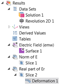
After computing the solution to a 2D axisymmetric problem, COMSOL Multiphysics automatically produces a revolution of the 2D data set called “Revolution 2D”, which is listed under “Data Sets”, as shown below.

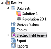
The revolved data set can be used in 3D plots. For the plots that we’re interested in, we’ll make a complete revolution from 0 to 360 degrees. The settings for “Revolution 2D 1” are shown below. You can see that under “Revolution Layers”, the start angle is set to 0 and the revolution angle is set to 360.

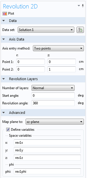
The coordinates for the plane in the 2D axisymmetric calculation are (r,z). The angle \phi is not defined since it is not part of the computational domain. However, it can be added as a coordinate in the 3D data set by checking the box beside “Define variables”. The variable name for the angle in the “Revolution 2D 1” data set is “rev1phi”. This can be used in expressions for plots and derived values, which we’ll do below.

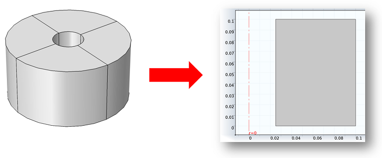
Consider an axisymmetric resonant cavity with a rectangular cross section, shown below. Only the rectangular cross section is modeled in the 2D axisymmetric formulation.

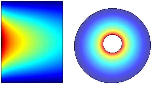
We can use an Eigenfrequency study to compute the resonant modes. Suppose that we would like to plot the field quantities for a mode with m = 1. The magnitude of the electric field is plotted in the rz-plane below on the left. Let’s also plot the magnitude of the electric field on a surface that bisects the cavity. This is done with a 3D Slice plot of “emw.normE” in an xy-plane where the number of planes is set to 1. The magnitude of the field is plotted below on the right. It is axially symmetric since the field is a traveling wave rotating about the z-axis, which also follows since | e^{j(\omega t – m \phi)} | = 1.

Plotting the Electric Field’s Radial Component

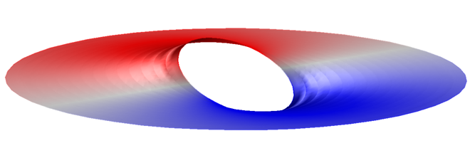
Now let’s plot the real part of the radial component of the electric field in the plane that bisects the cavity. Specifically, we want to plot Re \{ E_r(r,z) \, e^{j(\omega t-m \phi)} \} at t=0, where m=1. To get the angular dependence, we can use the variable “rev1phi” that was defined above in the Revolution 2D data set. In the expression field for the slice plot we’ll enter “Er*exp(-j*rev1phi)”. The color table for the Slice plot is set to Wave. Let’s also deform the Slice plot in the z-direction by an amount that is proportional to that quantity. We can do this by adding a Deformation node to the Slice node that is already there. The expression field for the z-component of the deformation plot contains the same quantity “Er*exp(-j*rev1phi)” and the other components are 0.

The plot of the radial component of the electric field is shown below. Note that this quantity is complex and that by default COMSOL plots the real part. This is equivalent to entering “real(Er*exp(-j*rev1phi))”. The imaginary part could be plotted by entering “imag(Er*exp(-j*rev1phi))”.

Generating an Electric Field Arrow Plot in 3D

Next up, we’ll make a 3D arrow plot of the electric field. The expressions for the Arrow Plot require the Cartesian components of the field whereas the dependent variables in the axisymmetric model are the cylindrical components. For this plot, we’ll use the variable “rev1phi” to convert the cylindrical vector components to Cartesian and also to account for the angular variation of the field in the Revolution 2D data set as we did above. The expressions for the Arrow Plot are listed below.

• x-component: (Er*cos(rev1phi)-Ephi*sin(rev1phi))*exp(-j*rev1phi)
• y-component: (Er*sin(rev1phi)+Ephi*cos(rev1phi))*exp(-j*rev1phi)
• z-component: Ez*exp(-j*rev1phi)

The grid for the arrow positions is 25 \times 25 \times 1.

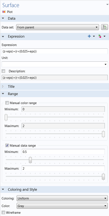
Let’s also add the lower surface of the cavity and the inner cylinder to the plot to provide some background for the electric field arrows. One way to do this is by including a uniform gray Surface plot on the lower surface z = 0 and on the inner cylinder r = 0.025. This is accomplished using conditional statements in the expression for the Surface plot, for example, “(z<eps)+(r<(0.025+eps))”, where “eps” is the machine precision. Since the expression is non-zero on the surfaces of interest, then in the settings for the Surface plot the data range is manually set so that the minimum value is 0.5 and the maximum value is 2, as shown below.

Animating the Plot

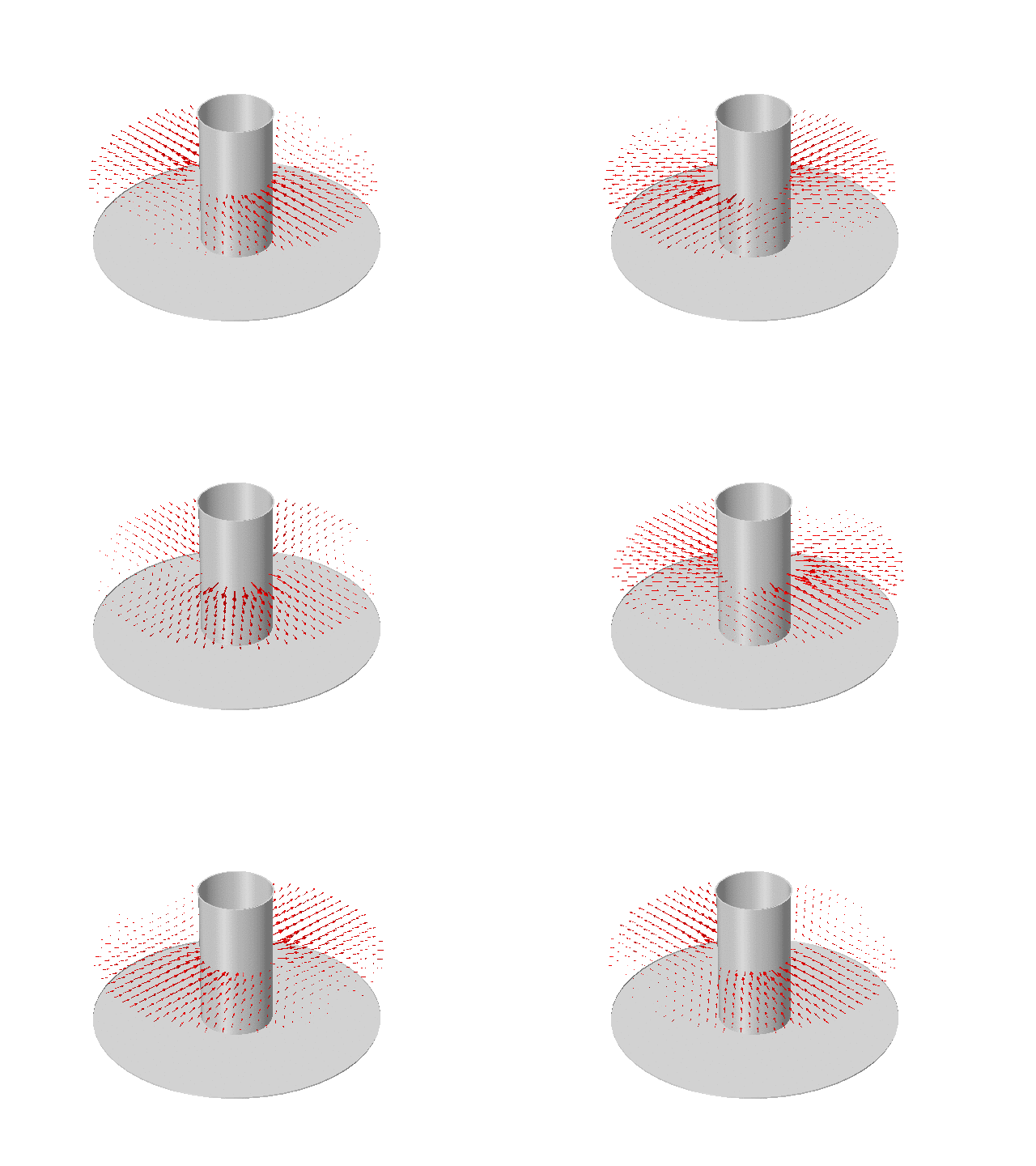
Finally, this plot is turned into an animation using the “Player” or “Animation” features. Both are found under Export in the model tree. Player creates an animation to view in the COMSOL graphics window, while Animation writes it to a file. To make a frequency domain data set oscillate in time, the sequence type is changed to dynamic data extension. Below you can see the electric field rotating about the z-axis: