
If you’re an engineer or researcher running electromagnetics simulations, the first multiphysics coupling you’re likely interested in is electromagnetic (EM) heating. Whether heating is the goal or an unwanted result of EM loss, the performance of an electrical device is almost always affected by temperature. Here, we discuss how to implement electrothermal analysis in both the low- and high-frequency regimes using built-in study types within the EM interfaces of the COMSOL Multiphysics® software.
Accounting for Sources of Electromagnetic Loss
There are many different sources of electromagnetic loss. With COMSOL Multiphysics, you can access built-in features to account for all of these EM heat sources, whether in the quasistatic or high-frequency regimes. The predefined interfaces include Joule Heating, Induction Heating, Microwave Heating, and Laser Heating.
Joule Heating
The Joule Heating multiphysics interface couples the Heat Transfer in Solids interface with Electric Currents (AC/DC Module). It considers heating due to conduction currents and dielectric loss.
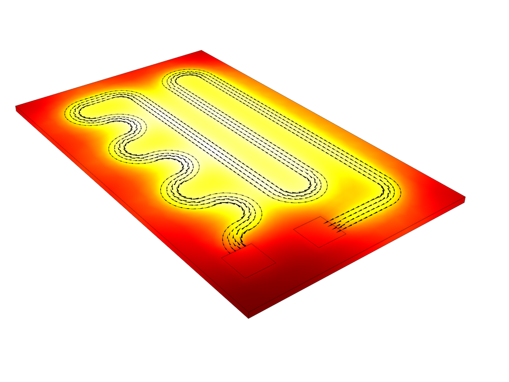
A resistive device modeled using the Joule Heating interface.
The heat source is added as Q_{e}=Q_{rh}, where Q_{rh}=\frac{1}{2}Re(\bold{J}\cdot\bold{E^*}) in the frequency domain or Q_{rh}=\bold{J}\cdot\bold{E} in the time domain.
In the frequency domain, the material properties representing loss are conductivity (σ) and complex relative permittivity (ε”):
\bold{J}=\sigma\bold{E}
\bold{D}=\epsilon_0\epsilon_r\bold{E}=\epsilon_0(\epsilon_r’-j\epsilon_r”)\bold{E}
Induction Heating
The Induction Heating multiphysics interface couples the Heat Transfer in Solids interface with Magnetic Fields (available in the AC/DC Module). It considers heating due to induced currents and magnetic losses.
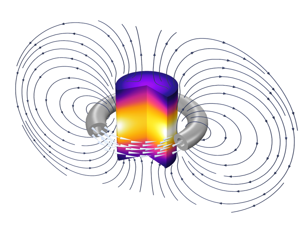
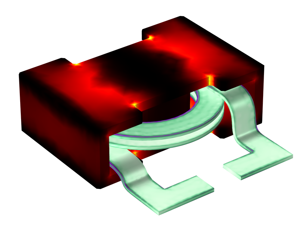
A ferromagnet core within an AC coil modeled using the Induction Heating interface.
The heat source is added as Q{e}=Q_{rh}+Q_{ml},where Q_{rh}=\frac{1}{2}Re(\bold{J}\cdot\bold{E^*}) and Q_{ml}=\frac{1}{2}Re(i\omega\bold{B}\cdot\bold{H^*}) in the frequency domain or Q_{rh}=\bold{J}\cdot\bold{E} and Qml depends on the hysteresis model in the time domain.
In the frequency domain, the material properties representing loss are conductivity (σ) and, for a linearized analysis, complex magnetic permeability (µ”):
\bold{J}=\sigma\bold{E}
\bold{B}=\mu_0\mu_r\bold{H}=\mu_0(\mu_r’-j\mu_r”)\bold{H}
Microwave Heating
The Microwave Heating multiphysics interface couples the Heat Transfer in Solids interface with Electromagnetic Waves, Frequency Domain (available in the RF Module). It considers heating due to resistive, dielectric, and magnetic losses in the high-frequency regime.
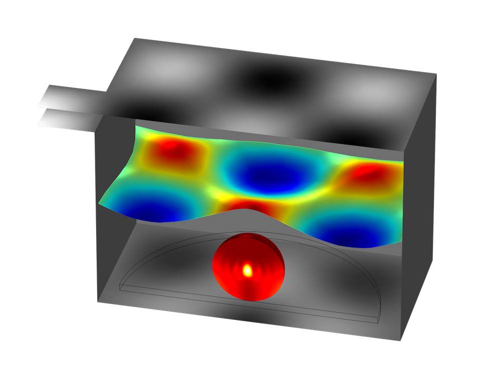
A microwave oven modeled using the Microwave Heating interface.
The heat source is added as Q_{e}=Q_{rh}+Q_{ml}, where Q_{rh}=\frac{1}{2}Re(\bold{J}\cdot\bold{E^*}) and Q_{ml}=\frac{1}{2}Re(i\omega\bold{B}\cdot\bold{H^*}) in the frequency domain. In the frequency domain, the material properties representing loss are conductivity (σ), complex magnetic permeability (µ”), and complex relative permittivity (ε”), as shown.
Laser Heating
The Laser Heating multiphysics interface couples the Heat Transfer in Solids interface with Electromagnetic Waves, Beam Envelopes (available in the Wave Optics Module). It considers heating due to resistive, dielectric, and magnetic losses in the high-frequency regime.
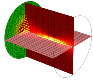
An incident Gaussian beam modeled using the Laser Heating interface.
The heat source is added as Q_{e}=Q_{rh}+Q_{ml}, where Q_{rh}=\frac{1}{2}Re(\bold{J}\cdot\bold{E^*}) and Q_{ml}=\frac{1}{2}Re(i\omega\bold{B}\cdot\bold{H^*}) in the frequency domain. In the frequency domain, the material properties representing loss are conductivity (σ), complex magnetic permeability (µ”), and complex relative permittivity (ε”), as shown.
The frequency-domain formulations for all multiphysics interfaces are shown here. Also shown are the time-domain formulations for the interfaces belonging to the low-frequency regime (AC/DC Module).
Dielectric losses (given by ε” term) are included in the Joule Heating interface for completeness, although this form of loss typically only becomes significant in the high-frequency regime.
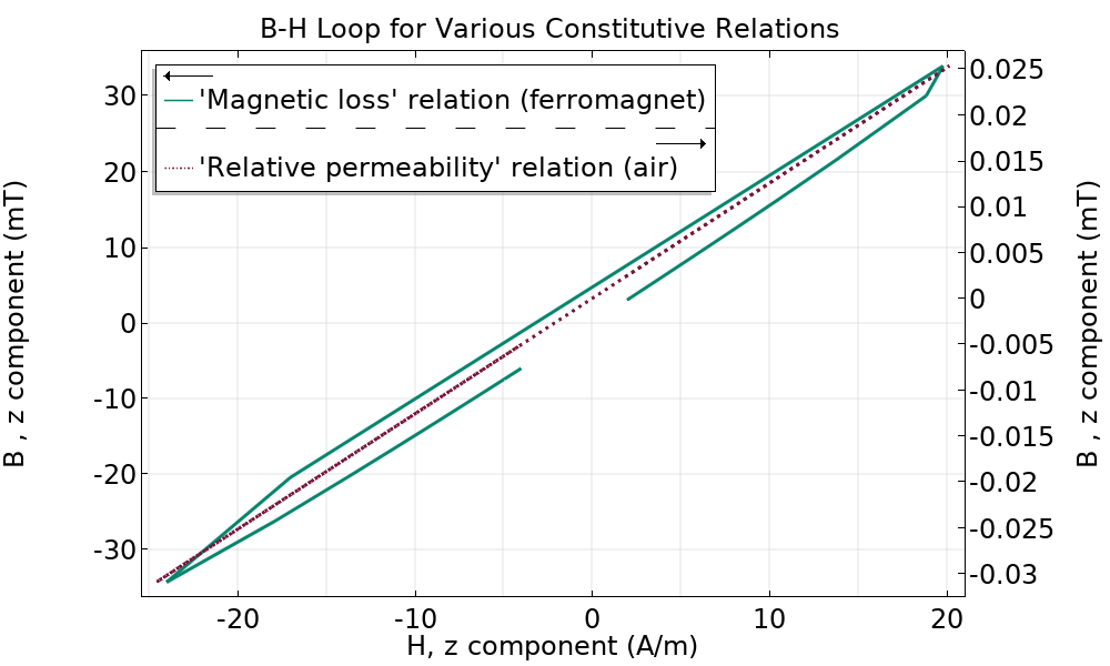
Magnetic losses within a material depend on the nonlinear relationship between B and H. This loss is most completely described via a full hysteresis loop in the time domain, however, the μ” term is a convenient way to quantify hysteresis loss in the frequency domain (see the figure below). For time-domain simulations with significant hysteresis loss, the Hysteresis Jiles-Atherton model option is available as a constitutive relation in the first physics subnode.
The default constitutive relation for a magnetic field model is Relative permeability. In the 3D Inductor tutorial, the air domain uses the default relation, with a constant and real-valued permeability of 1. Plotting Bz against Hz at a point within the air domain shows linear dependence. The ferromagnetic core uses the Magnetic losses constitutive relation with a complex component of permeability, which serves as a measure of hysteresis loss. Plotting at a point within the core domain shows the B-H curve take an elliptical shape, characteristic of hysteresis loops.
An Important Consideration for Electrothermal Analysis: Time Scales
A major advantage of AC excitation, from a simulation standpoint, is the ability to solve via a stationary formulation in the frequency domain with complex-valued solutions. The problem is that we likely want to observe the temperature rise in our device as a function of time. We might even have electrical properties that vary with time or temperature. Does this mean we can only model EM heating using a transient study type?
Solving the time-harmonic EM problem with a transient formulation is quite computationally costly compared to the alternative. Even more importantly, these costs become multiplied if we consider that EM cycles occur over ms or ns, while temperature rise may take minutes or hours! How can we expect to solve such problems in a reasonable amount of time?
Using the built-in study types in the COMSOL® software, we do not need to solve a fully transient problem at all. This is made possible by a sequential or segregated approach. If we can assume that the electromagnetic cycle times are short compared to thermal timescales, we can break the problem down into steps. The first step is to compute the EM losses. For AC signals, we can solve the EM problem in the frequency domain to get the cycle-averaged losses. In the second step, these losses are plugged in as a constant source of heat in a stationary or time-dependent heat transfer problem.
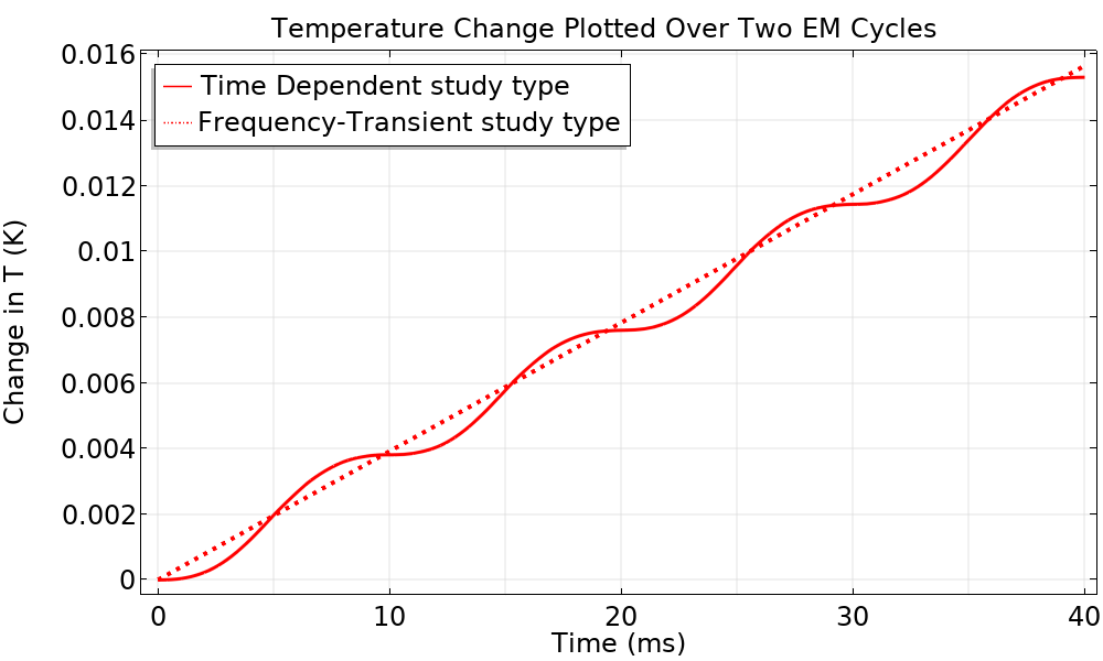
Left: Comparing temperature solutions between fully transient and frequency-transient study types over two EM cycles. We see that the time-dependent solution picks up small oscillations in temperature, but both solutions follow the same overall trend. Right: The Joule heating of a simple resistor is solved in two ways: using a fully time-dependent study type and using a frequency-transient study type. The first case allows us to plot the current and electromagnetic loss as a function of time. In cases where the EM cycle times are short compared to thermal time scales, a fully transient approach is computationally expensive and unnecessary. Instead, we obtain the cycle-averaged EM losses in the frequency domain and use these values as a continuous source of heat in a transient heat transfer problem.
Choosing a Study Type for a Time-Harmonic EM Heating Problem
For time-harmonic EM heating problems, we can choose from four study types:
- Frequency-Stationary
- Frequency-Transient
- Frequency-Stationary, One-Way Coupled, Electromagnetic Heating
- Frequency-Transient, One-Way Coupled, Electromagnetic Heating
What’s the difference between the first two types and their sequential counterparts?
Sequential study types are strictly a two-step process, and the best choice when there is a one-way coupling between the physics. In this case, the EM problem is solved in the frequency domain and cycle-averaged losses are computed. The losses are plugged in as a heat source in a subsequent stationary or transient heat transfer study. Sequential study types will use up less time and computational resources.
Frequency-Stationary and Frequency-Transient study types are more general and can handle some more complexity, such as temperature-dependent material properties. These studies use a segregated approach, moving back and forth between the EM and heat transfer problems until the convergence criteria has been met. The software uses an adaptive time stepping scheme, described here, to compute the solution over time.
Of course, we’ve used many relative terms here. What temperature rise is considered large enough? What is considered a significant change in material properties? This is determined by the relative tolerance specified in the study settings. Depending on the desired accuracy, the default tolerance value is usually a good place to start, and may be even tighter than what is needed. The default physics-controlled mesh is also suitable, as the software takes an educated guess on element type and size based on the physics and study settings. For example, in wave EM problems, the software automatically determines the wavelength (in each material) at the frequency entered in the study node and sizes accordingly, following the recommended criteria of at least five elements per wavelength. While the automated settings serve as a great starting point, note that a tolerance refinement study, in addition to the usual mesh refinement study, is needed to verify results.
The Microwave Oven tutorial model is an example of a one-way coupled problem, as it does not include any temperature-dependent material properties. Compared to the Sequential approach, the Frequency-Transient study type uses more than twice the amount of memory. While both studies reach the same solution, the Frequency-Transient study takes over four times longer to solve.
The RF Heating tutorial model, on the other hand, is an example that requires the segregated approach. This model has two temperature-dependent material properties:
- Thermal conductivity
- Loss tangent, loss angle
One of these properties makes it necessary to have a two-way coupling; can you guess which one?
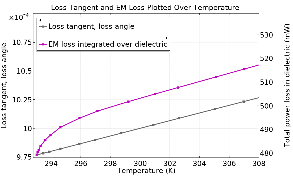
Left: The RF Heating tutorial is an example of a two-way coupled problem. The loss tangent, loss angle (δ) material property is required to compute the EM losses, but it varies linearly as a function of temperature as \delta=0.001*(\frac{T}{300 K}). The EM loss acts as a source of heat, which increases the value of temperature-dependent δ. In turn, an increased δ causes a rise in EM loss, and this cycle repeats itself until steady state is reached. Right: Ez variation plotted over phase, with the volume plot of the dielectric showing the magnitude of EM loss at a fixed time of 120 minutes. The EM cycles occur over a period of 0.1 nanoseconds.
The thermal conductivity belongs to the heat transfer part of the problem, so a one-way coupling here would be fine. The loss tangent belongs to the EM problem, but varies with the temperature solution of the heat transfer problem; this makes it necessary to have a two-way coupling.
The total EM losses and temperature within the dielectric plotted over time, with solutions stored at the steps taken by the solver. Both loss and temperature rise with time and then stabilize as the system approaches steady state. A Frequency-Stationary study reveals that the steady-state temperature is about 328.3 degrees Kelvin.
Whether we’re interested in a transient or steady-state solution for the temperature profile, this codependence between physics can be accounted for by selecting the appropriate study type. Now that we’ve discussed study types for AC heating, let’s discuss assumptions we can make to reduce the computation time for heating due to DC current.
Study Considerations for Problems Involving DC Current
By default, the equation form of a physics interface is set to Study controlled. This means that for a time-dependent EM heating study, the electric currents equation will have a time-dependent form, which includes the time derivative of the electric displacement field. In many cases involving current flow in good conductors, the ∂D/∂t term is negligible, and we can save computational resources by excluding it from our equations altogether. To do so, we can navigate to the Electric Currents (ec) node’s Settings window and force the equation form to Stationary.
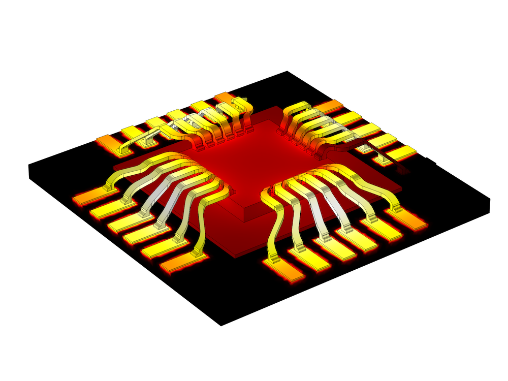
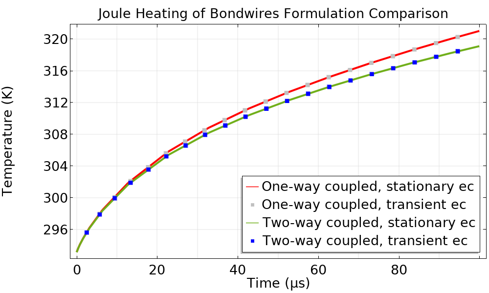
To compare the differences in simulation requirements between equation form settings, we consider a Joule heating study of bond wires arranged on a chip. We run both the one-way coupled problem (with no temperature-dependent material properties) and the two-way coupled problem (with a temperature-dependent Linearized resistivity conduction current model). In both cases, the two formulations reach the same solution, but when the electric currents problem uses a stationary formulation, the simulation takes less time and uses less memory. While this is a relatively light problem computationally, the advantages of using a stationary electric currents formulation (when possible) are only multiplied for larger problems.
The temperature profile is plotted on the 3D geometry, and the maximum temperature evaluated using various formulations is plotted. The “ec” term refers to electric currents (formulation).
Concluding Remarks
This blog post is an introduction to the various study types available to make electrothermal analysis simple. In the case of an AC current, the Frequency-Stationary, One-Way Coupled, Electromagnetic Heating and Frequency-Transient, One-Way Coupled, Electromagnetic Heating study types are the preferred choice for solving one-way coupled problems. Frequency-Transient and Stationary study types, on the other hand, are equipped to handle two-way couplings.
In the DC case, we can often neglect the time-dependent term in the electric currents equation and still obtain an accurate temperature solution; by doing so, we use less time and computational resources.
Regardless of how much complexity you ultimately decide to include, keep in mind that it’s always best to start with a one-way coupled problem to make sure the model is up and running before introducing temperature dependence. By working in steps, you can identify and correct potential sources of error more efficiently. Happy modeling!
Next Steps
If you have any EM heating modeling questions, feel free to contact our Technical Support team here:
Read more about electromagnetic heating on the COMSOL Blog:





Comments (0)