
Getting the Stats: Computing Standard Deviations and Other Statistical Quantities
Statistical quantities such as the standard deviation and mean value of a dataset can be valuable when you are assessing the performance or characteristics of a device, system, or process that you have simulated using the COMSOL Multiphysics® software. In this blog post, we will take a look at the functions, plots, and other tools that are available in COMSOL Multiphysics for computing and visualizing statistical quantities.
Statistics: An Overview
Statistics is about computing values that represent or visualize the values and variation of data. The following table lists some of the most common statistical measures with their operator and dataset operation names in COMSOL Multiphysics:
| Measure | Parameter | Operator Name | Dataset Operation Name |
|---|---|---|---|
| Mean or average | \mu | mean, timeavg |
Average |
| Standard deviation | \sigma | stddev |
Standard deviation |
| Variance | Var, \sigma^2 | – | Variance |
Here’s an overview of each of these statistical measures:
- The mean, average, or arithmetic mean (\mu in the equations below) is the sum of all data values divided by the number of values in the dataset. It is a useful value for characterizing the level of some fluctuating quantity. The mean can be sensitive to so-called outliers (that is, data values that differ significantly from the other values in the dataset). A related statistical quantity is the median, which is the middle value that separates the higher half from the lower half of the dataset (or the mean of the two middle values if the dataset contains an even number of values). The
timeavgoperator in COMSOL Multiphysics computes the average of a time-dependent expression over a time interval. - The standard deviation (\sigma in the equations below) tells you how much the data deviates from the actual mean. It is the square root of the variance. Contrary to the variance, the standard deviation is expressed in the same units as the data itself.
- The variance (Var in the equations below) measures how far a set of data values are spread out from their mean and is expressed in the units of the data squared.
The following equation shows the definition of the mean \mu:
The next equation defines the variance:
where X is the variable for which you want to compute the variance (and the mean), x_i are the set of values that it takes, and \mu is the mean. This definition of the variance is valid for fixed population of values.
In COMSOL Multiphysics, X and x_i represent a fixed set of values.
The standard deviation, \sigma, is simply the square root of the variance:
These statistical formulas can easily be generalized to describe statistical quantities defined on geometric entities where the summations are replaced by integration, which is the case in COMSOL Multiphysics. The integral form of an average of a variable X over a domain \Omega becomes
and, similarly, the variance of the variable X over a domain \Omega as
where |\Omega| is the size of the domain (volume, surface, or length, depending on the model’s space dimension).
The following sections explain how to use these operations and operators in COMSOL Multiphysics simulations.
Statistical Quantities in COMSOL Multiphysics
Nonlocal Coupling Operators
Later on we will see how to use the built-in operator stddev to compute the standard deviation of an expression. Before doing so, let’s see how to evaluate the average of a computed quantity, for example in a domain or along boundaries: Right-click the Definitions node under the Component node of interest, and then choose Average from the Nonlocal Couplings menu. Doing so creates an average operator, aveop1 by default, and in its settings you first define the Geometric entity level (Boundary, for example) and then the boundaries (or other geometric entities, depending on the chosen entity level) for which you want to evaluate the average. You can also add operators in the same way for computing integrals, maximum values, and minimum values.
You can use the operators you have created in a model and during postprocessing. For example, in a fluid flow simulation, you can use an average operator defined on the outlet boundary to compute the average outflow velocity. To do so, in a Global Evaluation node under Derived Values in the Results section, add an expression like aveop1(spf.U) and then click Evaluate. The average velocity for each output time in a transient simulation then appears in a Table window.
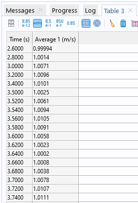
A Table window with the values of the average velocity for each output time.
You can compute a standard deviation or variance using a nonlocal coupling operator twice: once to compute the average and once to compute the standard deviation or variance itself. For example, using the average operator aveop1 defined for the outlet boundary in our fluid flow example, you can compute the standard deviation using a Global Evaluation node and the expression sqrt(aveop1((aveop1(p)-p)^2)), which implements the equations above for the standard deviation of the pressure on the boundary.
Simplifying Using an Expression Operator
The expression above, sqrt(aveop1((aveop1(p)-p)^2)), is a bit long, so if you want to use it in several places, you can define an Expression Operator to simplify it. First, you need to enable Variable Utilities under the General section in the Show More Options dialog box. Then you can add an Expression Operator node from the Variable Utilities submenu that appears when you right-click the Definitions node under Component. In the settings for the Expression Operator node, you define an operator, called stdop1 for example, with an expression like the one above but with an input argument of your choosing, say pin, as in the following image:
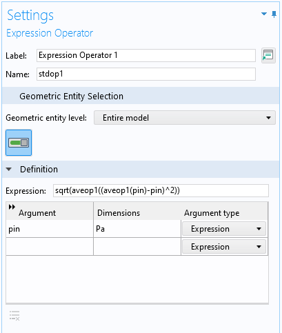
The Settings window for an Expression Operator node, defining a simplified operator, stdop1, for the standard deviation.
You can then use this operator during postprocessing, typing stdop1(p) instead of sqrt(aveop1((aveop1(p)-p)^2)).
Derived Values
For postprocessing purposes, you can add Volume Average, Surface Average, and Line Average nodes, which you implement by right-clicking the Derived Values node and then choosing one of these options from the Average submenu. You can define similar nodes for Integration, Maximum, and Minimum values.
Transformations of Time Series and Parametric Sweeps
When evaluating data from time-dependent, parametric, or eigenvalue solutions, using a Point Evaluation feature, for example, you can apply one of the following operations on the data series:
- Average
- Integral
- Maximum or minimum
- Root mean square (RMS)
- Standard deviation
- Variance
Each of these operations provides a single output, which may be the average of a value in a parametric sweep or the standard deviation of a quantity at a point in a time-dependent simulation.
Built-In Operators
When evaluating and plotting the results of a COMSOL Multiphysics simulation, you have access to a large number of physics-specific variables as well as built-in physical and mathematical constants, functions, and operators. You can type them directly into any Expression field or you can click the Add Expression or Replace Expression button (available in the Expression section toolbar in results features). The following screenshot shows the available operators in the Integration and statistics category as of COMSOL Multiphysics® version 6.0:
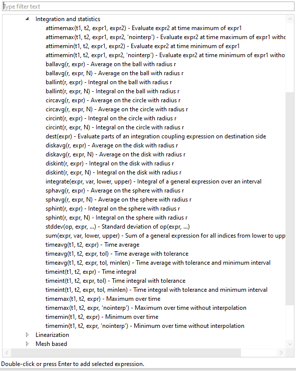
The available operators for integration and statistics.
Of special interest is the stddev operator, which you can use to compute the standard deviation of an expression. You can use it to evaluate the standard deviation for the same outlet boundary pressure case above using the expression stddev('comp1.aveop1',p), which is a more direct, efficient syntax than the nested call to the average operator used in the previous expression for the standard deviation. Note that the component and operator names given here are merely examples, and they can have other names in your models.
Standard Deviation and Mean: An Example
Let’s compute a couple of statistical values for the time-dependent Flow Past a Cylinder model, which can be found in the Fluid Dynamics folder in the Application Library in COMSOL Multiphysics. We will compute the following values:
- The average and standard deviation of the pressure in the computational domain for all time steps in the simulation
- The average and standard deviation of the velocity at a point at the outlet boundary, computed over all time steps
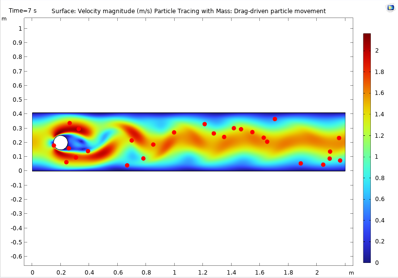
The default plot for the Flow Past a Cylinder model, showing the velocity field and particle movement at the end time of the simulation (7 s).
Average and Standard Deviaton of the Pressure in the Domain and on the Outlet Boundary
To evaluate the average and standard deviation of the pressure in the domain, first add an Average nonlocal coupling node, say aveop2, and define it in the domain. (There is only one domain in this geometry). After computing the solution, you can add a Global Evaluation node under Derived Values in the Results section to evaluate the average pressure using the expression aveop2(p). The average pressure is then displayed in a Table window for all times selected from the Time selection list. (The default is to include all time steps.) If you want to compute the average of the average pressure over all time steps, choose Average from the Transformation list in the Data Series Operation section. The output then is a single scalar number for the average of the average pressure. For the standard deviation at each time step, use the expression stddev('comp1.aveop2',p) (or either of the other options mentioned above).
The argument to the stddev operator does not have to be an average. Instead, you can pass it an integration coupling operator, for example, and it would still evaluate a correct standard deviation of the average. You could also use it in combination with the timeavg operator to produce the same results as you get in other places by using a data operation on the time series using an expression like stddev('timeavg',t1,t2,expr), where t1 and t2 are the start time and stop time, respectively, for the time interval, and expr is the expression to compute the time average for over that time interval. For example, to plot the time-domain standard deviation of the pressure in every point along the outlet boundary as a time-average value from 6 seconds to 7 seconds, use stddev('timeavg',6,7,p).
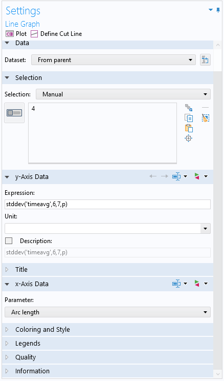
The Settings window for a Line Graph plot with the expression for a time-domain standard deviation as a time-average value from 6 seconds to 7 seconds.
The corresponding plot shows that the standard deviation of the pressure is smallest in the middle of the outlet boundary.
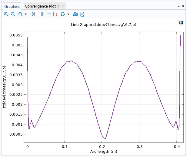
The Line Graph plot of the time-domain standard deviation at the outlet boundary.
Average and Standard Deviation of the Velocity at the Outlet
If you instead want to evaluate the average and standard deviation at the midpoint of the outlet boundary over all time steps, you must first ascertain the velocity at that point. You can do so using two methods:
- Add a point in the geometry at the middle of the output boundary, even if it is not needed for creating the geometry
- Add a Cut Point dataset (Cut Point 2D in this case) and then define the coordinates for the cut point in the settings for the dataset
To evaluate the velocity at the midpoint, use a Point Evaluation node and either select the point that you have defined or use the Cut Point 2D dataset as the input dataset (depending on the chosen method for the point data). Then use spf.U, for example, as the expression for the velocity magnitude. In the Data Series Operation section, choose Average and then Standard deviation, clicking Evaluate at the top of the Settings window after each selection to get the average and standard deviation (both in m/s) for the velocity magnitude at the midpoint of the outlet over all time steps in the simulation.

The average velocity magnitude and the standard deviation of the same quantity, displayed in a Table window.
Histogram Plot
Histograms are useful for illustrating the shape and spread of some data. The plotting tools in COMSOL Multiphysics include the following histogram plot types:
- Histogram (1D and 2D plots), which shows how a quantity is distributed over the geometry (i.e., mesh volume). In 1D histograms, the x-axis represents the values of the quantity (as a number of bins or a range of values), and the y-axis represents the count of the total element volume in each interval.
- Table Histogram (1D and 2D plots), which is similar to a Histogram plot but is based on data from a table or evaluation group.
- Matrix Histogram (2D plots only), which you can use when you have a precomputed matrix that you want to visualize as a 2D histogram.
For Histogram and Table Histogram plots, you can choose if you want to specify the number of bins in the histogram or if you want to specify a range of limits for the histogram bins. For any 2D histogram, you can add a Height Expression subnode to plot the magnitudes of the bins along the z-axis, as shown in the following 3D histogram.
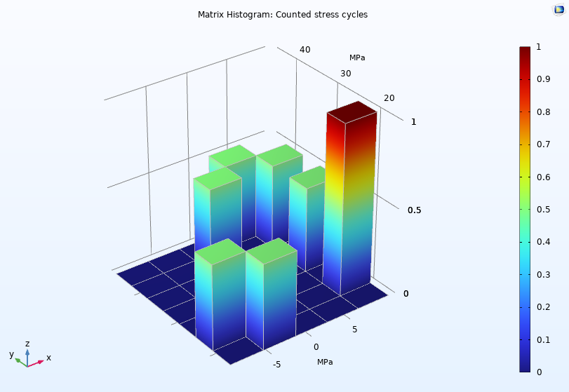
A Matrix Histogram plot visualizes counted stress cycles in the Cycle Counting in Fatigue Analysis — Benchmark model.
Uncertainty Quantification and Statistics
Using the Uncertainty Quantification Module, an add-on to COMSOL Multiphysics, you can access statistical data related to uncertainty quantification simulations directly in output table groups. For example, for an uncertainty propagation (UP) analysis using nonadaptive Gaussian process surrogate modes, the following four tables become available:
- A QoI Confidence interval table, which contains one row per quantity of interest (QoI), with columns for the mean, standard deviation, minimum, and maximum, followed by confidence intervals for 90%, 95%, and 99% likelihood.
- A UP predicted QoI table, which contains the surrogate-model-predicted values for the QoIs for the Monte Carlo sampling points.
- A UP predicted standard deviation table, which contains the surrogate-model-predicted standard deviation for the Monte Carlo sampling points. This can be seen as the built-in surrogate model error estimation.
- A Maximum entropy table, which contains the maximum relative standard deviation, one per QoI.
When an adaptive Gaussian process surrogate model is used, four corresponding adaptive result tables are also added to the output table group. They contain the result information at all of the adaption steps.
Next Step
As a next step, try some of these statistical tools in your own simulation models; in doing so, you can gain a statistical understanding and quantification of the variations and characteristics of variables or parameters of interest. If you have any questions related to this topic, contact COMSOL via the button below.


Comments (7)
Ivar KJELBERG
June 22, 2022Thanks Magnus for again an interesting BLOG, making me discover the (new ?) “Expression Operator” node. But, even after quite some reading of your latest documentation, I do not really get all the subtle differences (pros and cons) between an “Analytical Function” and this new operator, as well as exactly when to use one or the other. Any means, for you, to add a little there, or for a new BLOG ?
Sincerely,
Ivar
Magnus Ringh
June 22, 2022 COMSOL EmployeeHi Ivar,
Thanks for the kind words. Here is some more information about the Expression Operator, including some differences compared to an Analytic function:
– The Expression Operator was released with version 5.5.
– Contrary to an Analytic function, an Expression Operator can be defined to be active only in some domains, for example.
– An Expression Operator can be used as a convenient shorthand instead of more complex expressions, which you use to define the Expression Operator, as in this blog example.
– An Expression Operator can have different definitions in parts of the model geometry using Operator Contribution subnodes.
– It can be helpful to think about the Expression Operator as a parameterized Variable rather than an Analytic function.
– An Expression Operator can, in its definition, use any expression that can be evaluated where the Expression Operator is evaluated; an Analytic function, in contrast, should be a pure function of its arguments.
– An Analytic function can, thanks to its global nature, be used in the definition of model parameters; an Expression Operator cannot.
– We will consider a separate blog post about the Expression Operator.
Best regards,
Magnus
Roy Dai
October 25, 2023Hi Magnus, very nice blog. May I ask if there is any analytic method that we would be able to compute the RMSE or MAPE of simulation results vs imported experimental data? That would be really powerful!
Magnus Ringh
October 26, 2023 COMSOL EmployeeHi Roy, and thanks!
Currently there is no built-in method in COMSOL Multiphysics for computing the RMSE or MAPE, but it is something that we will consider for future versions.
Magnus Ringh
November 7, 2023 COMSOL EmployeeHi Roy, in COMSOL Multiphysics version 6.2, released today, it’s possible to add Comparison subnodes to graph plots to compare them with reference values in tables using RMS as one of the available metrics. That should be similar to your RMSE request, I think.
Best regards,
Magnus
Sinéad Mannion
September 17, 2024This is great, can you make a video of this please!!!
Evan Sisler
September 17, 2024 COMSOL EmployeeHi Sinéad,
Thank you for your comment! We will pass your suggestion on for consideration.