
Versions 6.0 and 6.1 of the COMSOL Multiphysics® software introduced major functionality improvements for buckling analysis. Version 6.0 introduced the ability to include geometrical imperfections in the analysis, and version 6.1 made it possible to separate fixed (“dead”) and varying (“live”) loads. In this blog post, we will explore these types of analyses in detail.
Editor’s note: Our previous blog post, “Buckling, When Structures Suddenly Collapse,” covered various aspects of buckling analysis and discussed some techniques for more specialized buckling analysis. The information provided there applies to those who use a version earlier than 6.0.
Including Geometrical Imperfections
It’s well known that for some structures, the load-bearing capacity, with respect to buckling, can decrease significantly due to geometrical imperfections. In real life, there are always some manufacturing defects in a structure. In addition, mounting during construction may be imperfect, or a structure may be deformed as an effect of service loading. Thus, it may be important to take imperfections into account.
There are different strategies for this. For a simple structure, like a single strut, you can postulate a certain geometric shape. If you want to include that in your model, you can either directly create the geometry including that imperfection or start with the ideal geometry and add a Deformed Geometry interface with a Prescribed Deformation node.
For a more complex structure, it’s often difficult to postulate a suitable imperfect shape. One solution is to perform a linear buckling analysis and then use one or several buckling modes as the imperfection. The reasoning behind this approach is that it’s probable that there’s a sensitivity to the buckling mode itself.
Note that when studying the effect of imperfections, you can generally not use a linearized buckling analysis. It’s necessary to increase the load incrementally until failure occurs. The deformation will be progressive, so the failure criterion is typically a maximum allowed displacement or stress.
As of COMSOL Multiphysics version 6.0, there is a method for automatically setting up a study based on buckling mode imperfections. Let’s take a look at setting up this study.
7 Steps for Setting Up a Study Based on Imperfections
Step 1: Start with Linear Buckling Analysis
You want to start with an ordinary linear buckling analysis of the ideal structure. If you’re going to include more buckling modes than the first one in the imperfection shape, you need to change the number of computed buckling modes from the default value of 1.
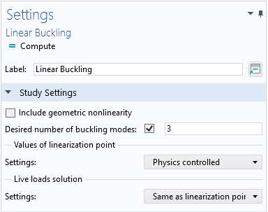
Changing the number of computed buckling modes.
Step 2: Add a Buckling Imperfection Node
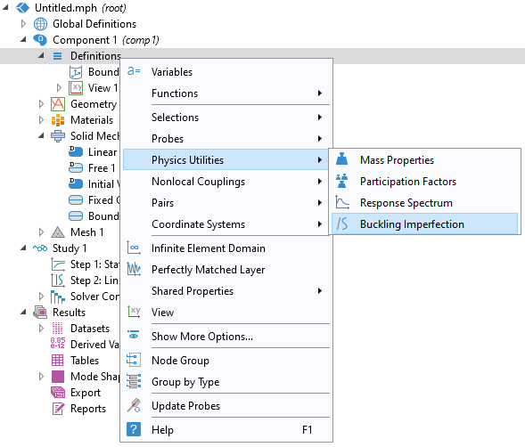
Now that the buckling modes and the corresponding critical load factors are available, the next step is to add a Buckling Imperfection node under Definitions.
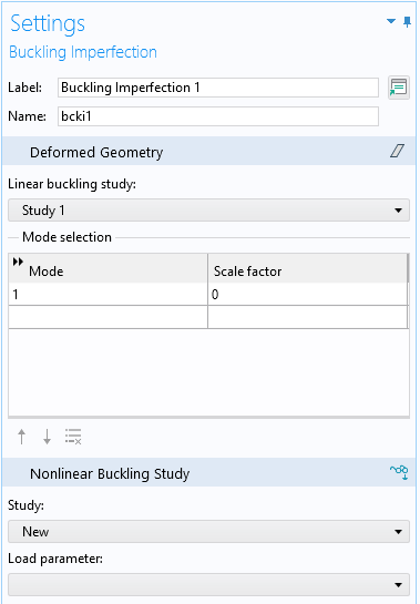
In the image on the left, we can see how to add a Buckling Imperfection node, while the image on the right shows the Settings window for the newly added node.
Step 3: Enter Mode Numbers and Their Scale Factors
We now need to adjust the settings of the Buckling Imperfection node you have added. This includes entering mode numbers and scale factors. To determine an appropriate scale factor, you first need to know the maximum deflection of the buckling mode. The amplitude of a buckling mode is arbitrary, so the solver applies some scaling. By default, the mode is scaled so that the maximum displacement is 10-6 times the length of the geometry’s diagonal bounding box.
The actual imperfection amplitude should reflect the geometrical quality of the real structure. Alternatively, the size of the imperfection may be given by some design code. Let’s assume that the real-world geometry can differ by 2 mm from the ideal shape and that the size of the geometry is 1 m. If you use a single buckling mode, the scale factor will be 2000. If you are using more than one mode, assigning a scale factor of 2000 to all modes may be on the conservative side since the values would sum up. This is not trivial, as some modes may act in opposing directions. You need to inspect the modes and possibly even assign negative scale factors to some of them to get the intended shape.
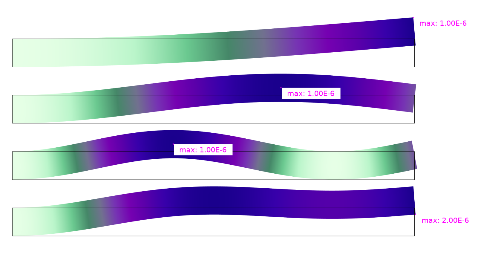
From top to bottom, the first three plots show the first three buckling modes for an Euler 2 column, while the plot at the bottom shows a pure superposition of these modes. The markers show the maximum vertical displacement. (You can try modeling this yourself by downloading the model’s MPH file, euler2_buckling_imperfection.mph, from the Application Gallery.)
Step 4: Configure the Deformed Geometry
Next, we will set up the deformed geometry. To do this, click the Configure button on the Deformed Geometry section header.
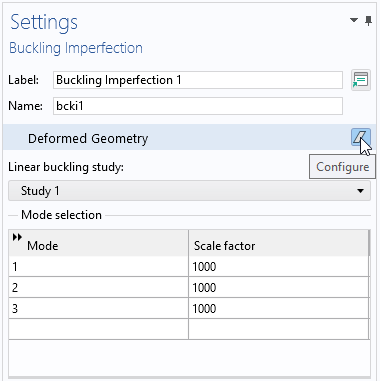
Creating the deformed geometry.
With this, a Deformed Geometry node with a specially configured Prescribed Deformation node is added to the Model Builder tree.
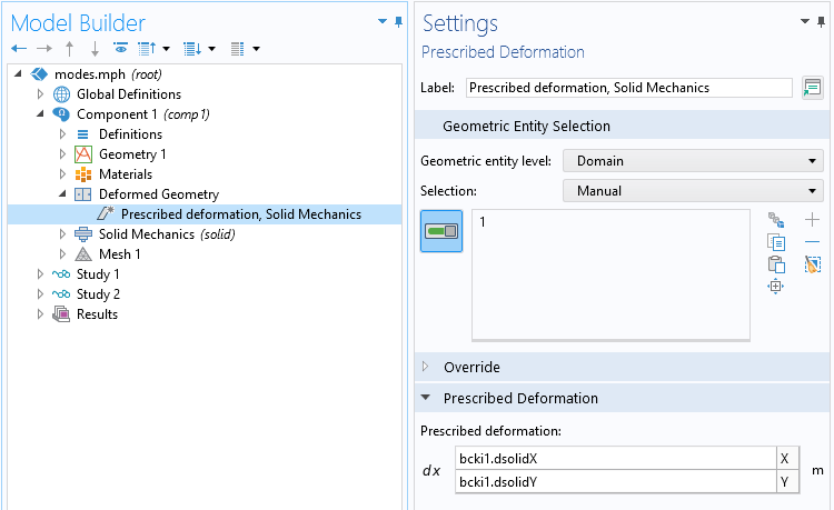
The new Prescribed Deformation node.
This step does not need to be repeated if you were to change the included modes, their scale factors, or ever rerun the linear buckling study.
Step 5: Create a Loading Parameter
Add a parameter that will act as a multiplier to the loads. Then insert that parameter in all load features used for the linear buckling analysis.
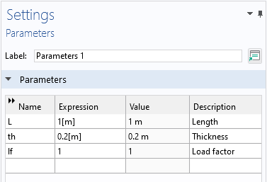
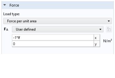
A new parameter, lf, has been added and used as the multiplier for all loads.
Next, select the If (Load factor) parameter in the Load parameter drop-down list.
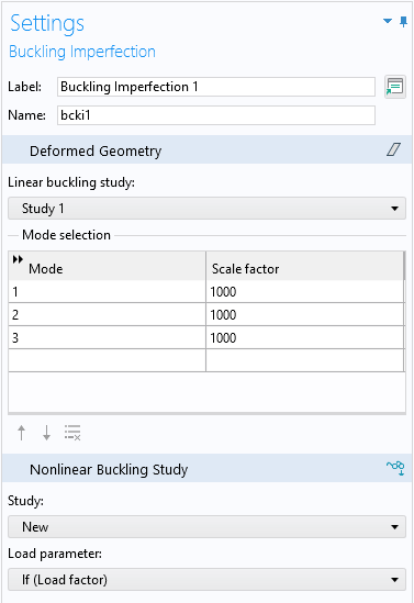
The load parameter is now selected.
Step 6: Configure the New Buckling Study
To create a study for the incremental analysis with the imperfection included, click the Configure button on the Nonlinear Buckling Study section header.
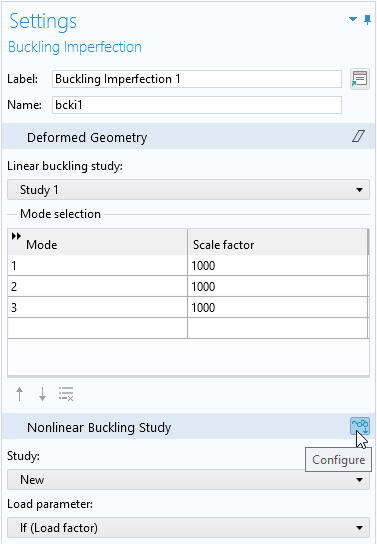
Creating the nonlinear buckling study.
A new study is created, with some special settings:
- Geometric nonlinearity is included.
- An auxiliary sweep is added using the selected load parameter.
- The parameters value list is based on the lowest critical load factor from the computed buckling modes. With these settings, the maximum load is about 10 percent above the prediction from the linearized buckling study.
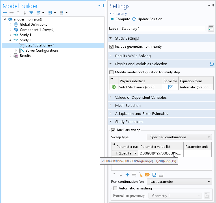
The Settings window for the new study.
Step 7: Run the Study
The study may fail to converge at the higher load levels. This will usually indicate that the limit load has been exceeded by far, but the intermediate steps are still stored and can be used for evaluation.
For a nonlinear buckling analysis, there is no unique critical load. Usually, you need to plot relevant displacement and stress quantities as a function of the load parameter and use a failure criterion based on the physical properties of the structure.
The example below is the same Euler 2 case used to indicate the three buckling modes above (a cantilever beam with a length of 1 m). Let’s say that the maximum allowed tip displacement is 10 mm, and that the maximum allowed von Mises equivalent stress is 400 MPa.
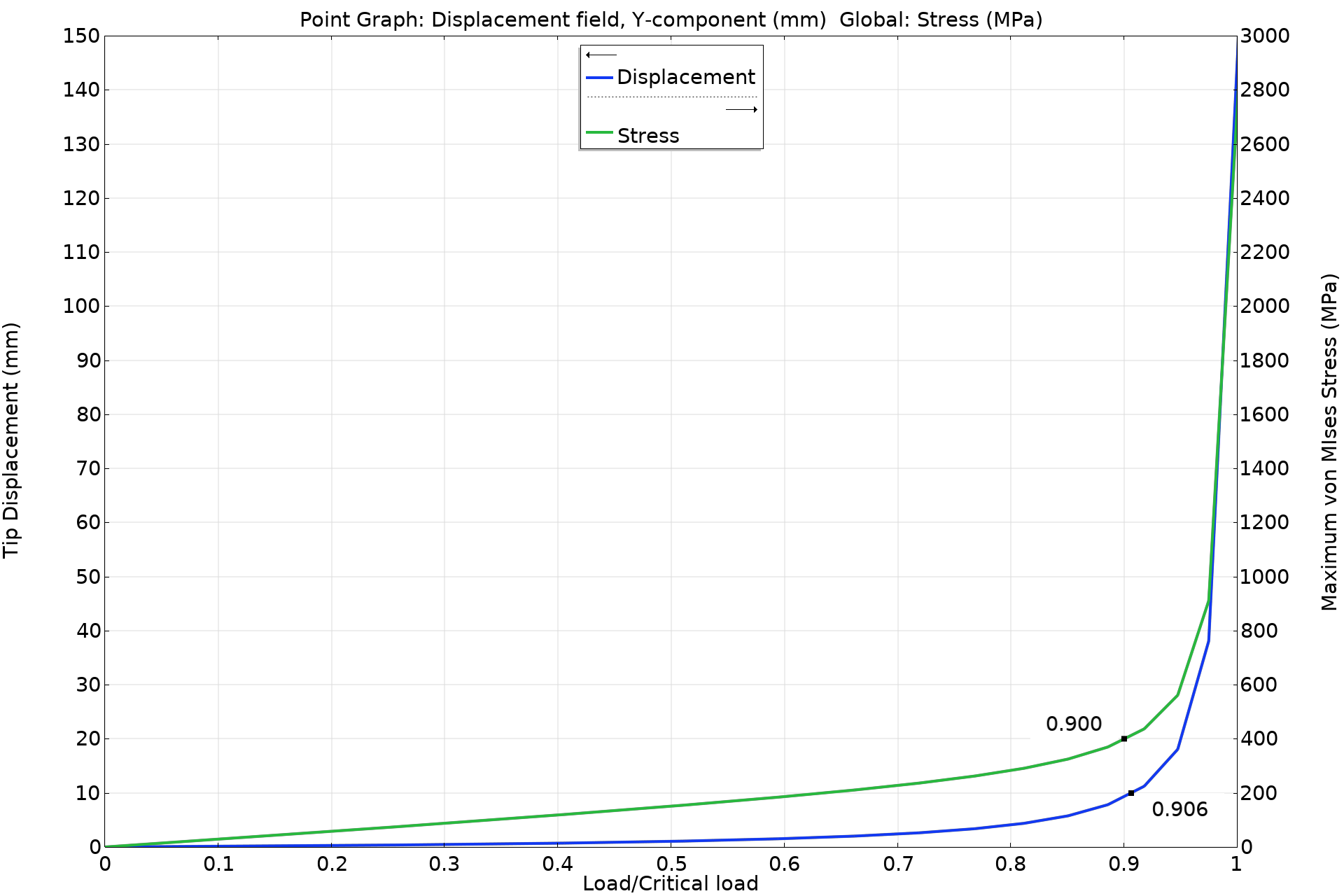
A graph showing the displacement and stress as functions of the load parameter. The critical load factor from the buckling analysis normalizes the horizontal axis. The graph markers indicate the criteria 10 mm and 400 MPa, respectively.
In the table below, a comparison of the critical load values is shown for different buckling mode scaling choices.
|
Scale factor, mode 1 |
Scale factor, mode 2 |
Scale factor, mode 3 |
Maximum imperfection (mm) |
Critical load (displacement) |
Critical load (stress) |
|---|---|---|---|---|---|
| 1000 | 1000 | 1000 | 2 | 0.906 | 0.900 |
| 2000 | -2000 | 2000 | 2 | 0.832 | 0.846 |
| 2000 | 0 | 0 | 2 | 0.906 | 0.900 |
| 1000 | 0 | 0 | 1 | 0.907 | 0.908 |
| 20000 | 0 | 0 | 20 | 0.326 | 0.451 |
It can be seen that for moderate levels of imperfection, the sensitivity to the actual choice of generating modes is limited.
This example was rather simplistic, and an Euler strut is not very imperfection-sensitive. Shells are usually more problematic in this respect, so next, we will explore such an example.
A More Advanced Example
In this example, we are looking at a steel cylinder with a diameter of 1.5 m and a height of 2 m. The thickness is 10 mm, and there are two stiffening rings with a thickness of 20 mm. An axisymmetric shell element is used for the analysis. (You can explore this model by downloading its related MPH file, cylindrical_shell_buckling_cleared.mph, from the Application Gallery.)
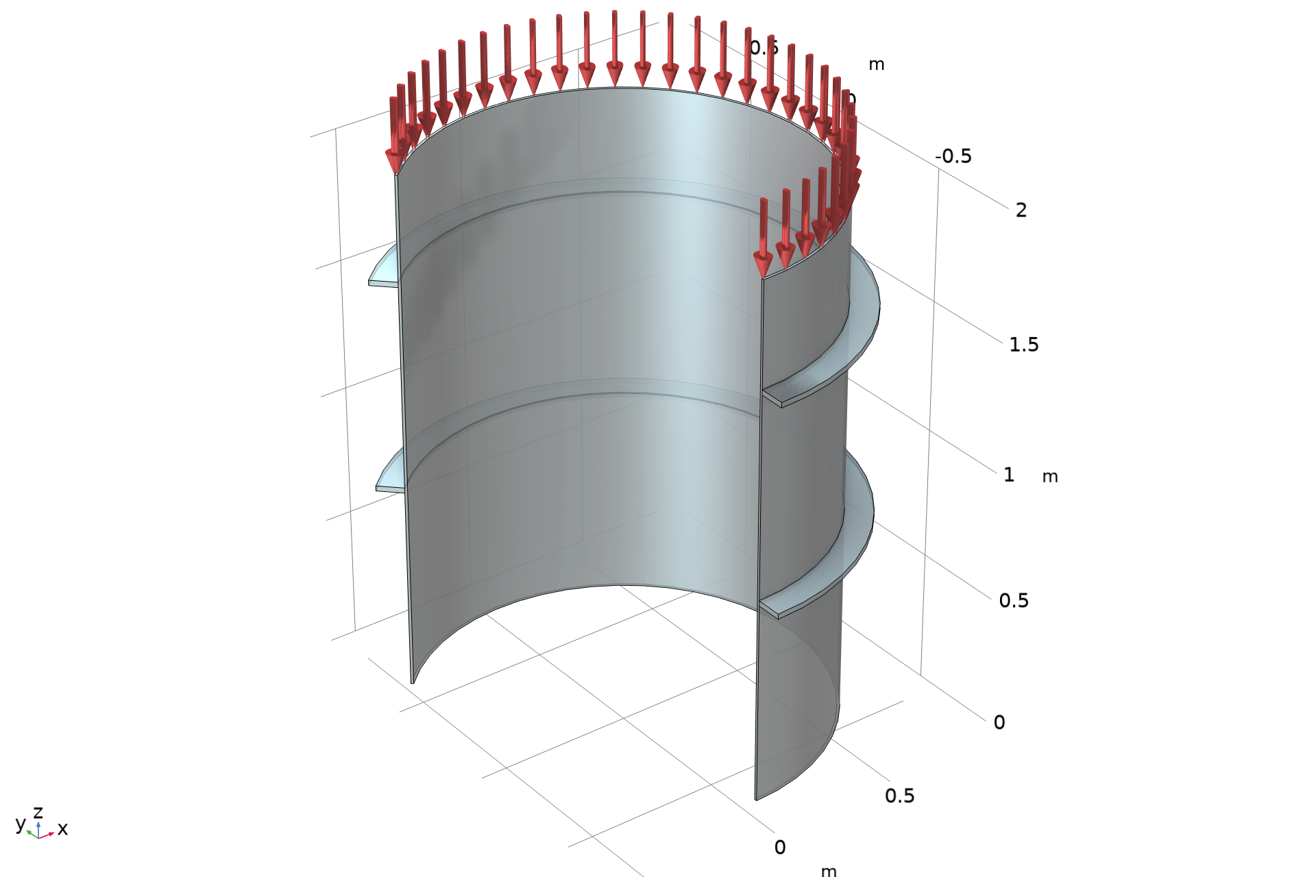
The geometry and loading. The lower end of the cylinder is fixed.
There are many buckling modes with similar critical load factors.
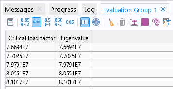
The critical load factors corresponding to the first five buckling modes.
In a situation like this, it’s important to check different imperfection patterns. It’s possible to automate this by adding an external parametric sweep over the mode numbers, as shown below.
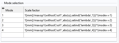
The Mode selection table in the Buckling Imperfection node.
When regarding the table, take the following information into account:
- The Boolean expressions of the type
(mode==1)act as a filter for which mode to use as an imperfection.modeis the sweep parameter. - The scale factor is designed so that the peak deformation for each mode is 1 mm.
maxop1is a maximum operator (added under Definitions → Nonlocal Couplings) used to get the maximum displacement in the radial direction for each buckling mode.- The purpose of the withsol operator is to pick results from a specific solution. In this case, it is used for retrieving individual buckling modes. (Learn more about this operator in our Learning Center article “Examples of the withsol Operator”.)
The nonlinear analysis now includes an outer sweep over the first four modes as imperfection and the same inner auxiliary sweep where the load is ramped up for each mode. Since any of the nonlinear solutions may fail to converge at higher loads, it’s essential to set up the parametric sweep so that the entire analysis doesn’t fail because of this.
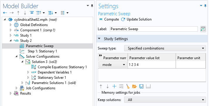
The nonlinear study and the Parametric Sweep node.
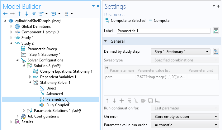
In the Parametric node, the On error option must be set to Store empty solution.
It’s now possible to plot the variation of the maximum stress and displacement for all the cases.
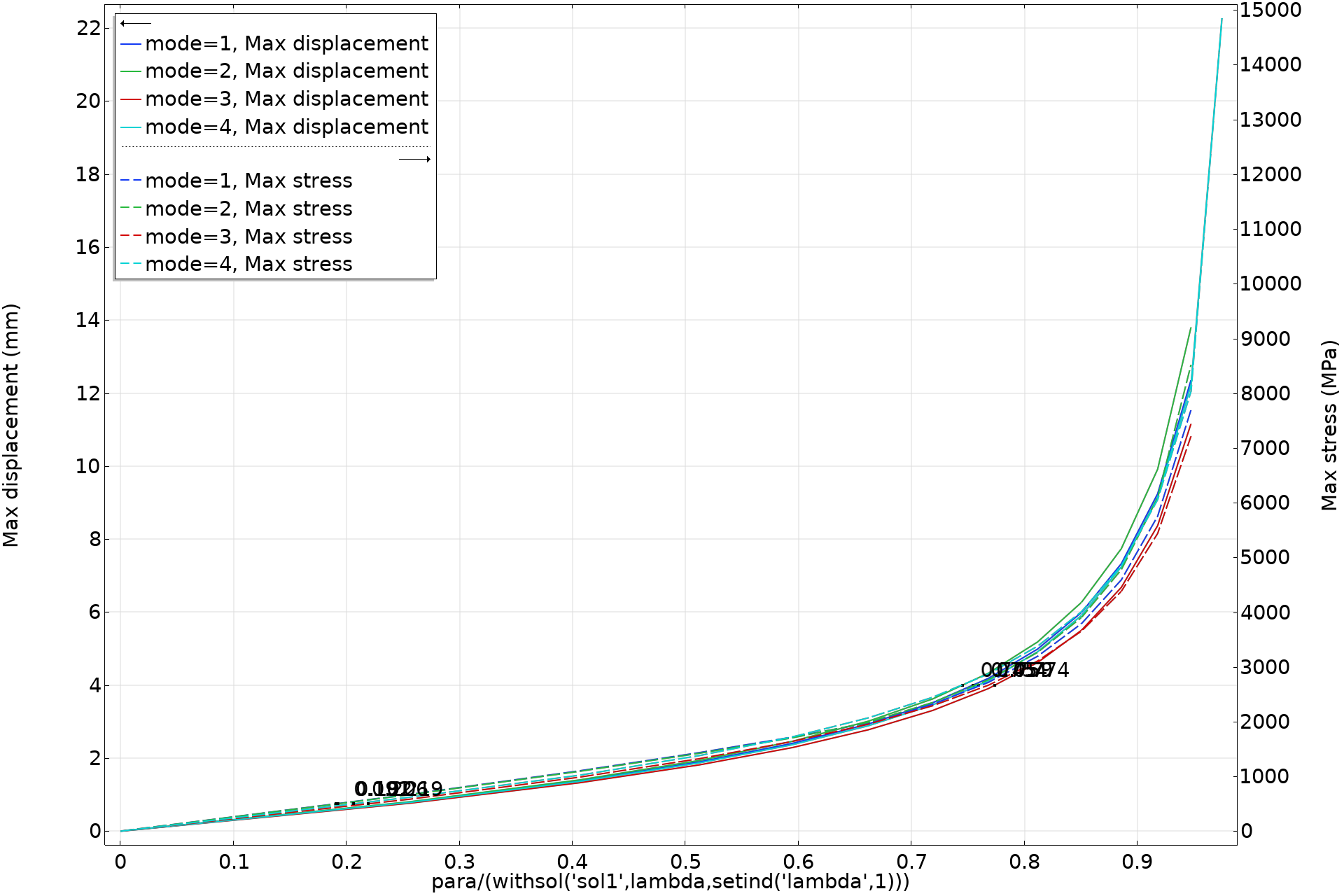
A graph showing the displacement and stress as functions of the normalized applied load.
In this case, the allowed stress is for all cases exceeded at a rather low external load. It occurs already in the linear region. The conclusion is that this structure will fail due to plastic collapse well before buckling occurs. It would be possible to refine the analysis by including plasticity in the model.
One exciting feature in this example is that, to a large extent, the deformation in the nonlinear analysis adapts to the suggested imperfect shape.
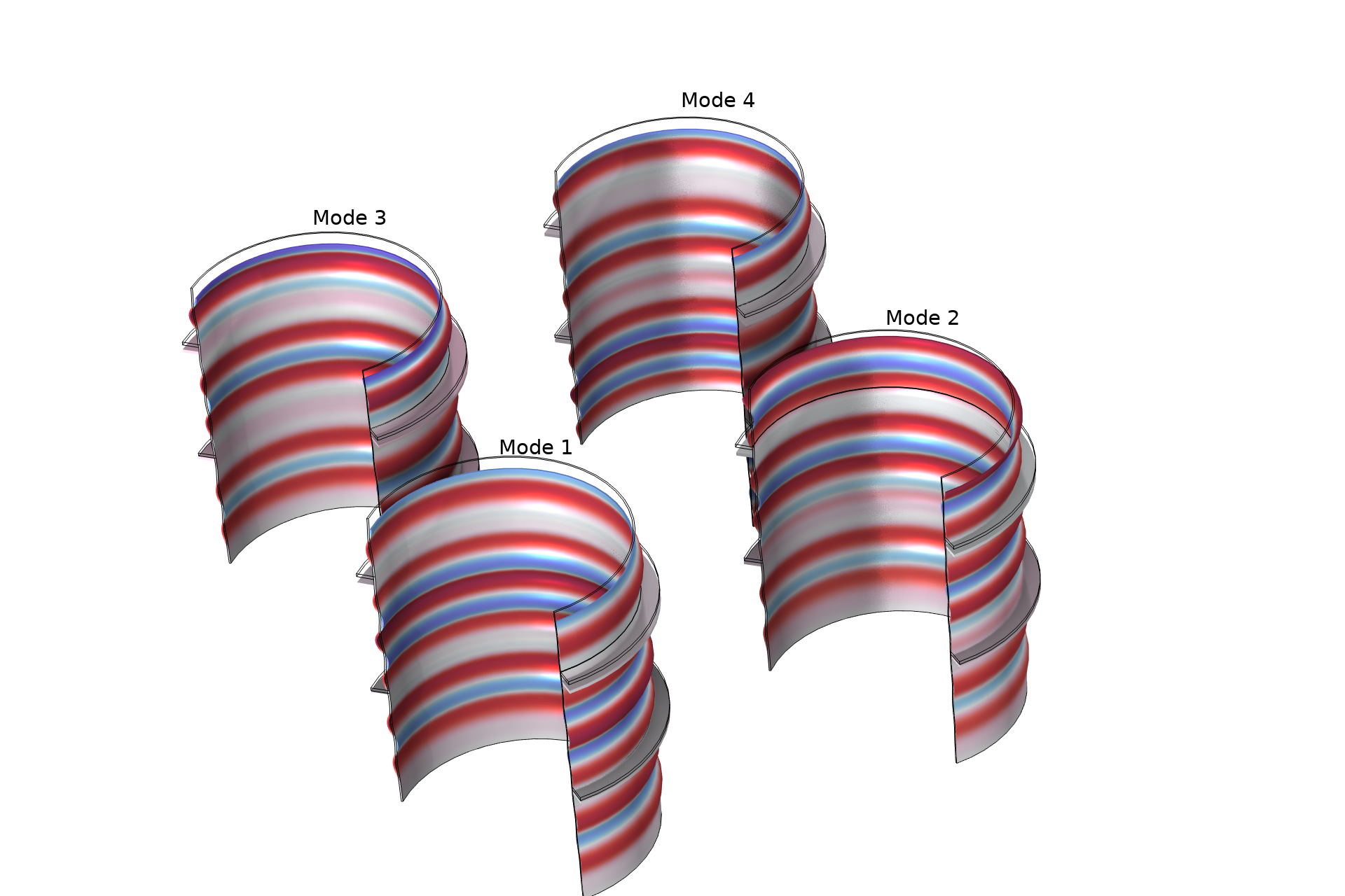
Deformed shape (scaled by a factor of 5) close to failure load for the different imperfections. The colors indicate the radial displacement.
It’s important to note that you cannot safely assume that all buckling modes of an axisymmetric shell are also axisymmetric. The true first buckling mode, which is not axisymmetric, looks like this:
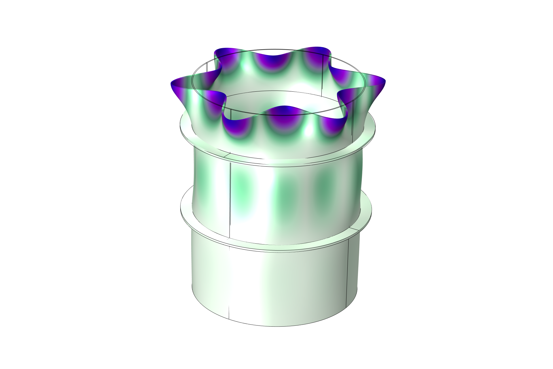
The first buckling mode when using a full 3D formulation.
Combinations of Live and Dead Loads
The load factor in a linear buckling analysis can be considered as a type of safety factor with respect to the applied load. Sometimes, only a certain set of loads can vary. Other loads have well-defined values, as is typically the case for self-weight. If we assume that the structure will not fail due to gravity alone, then the question to be answered is: What is the safety factor for the service loads, taken into account that part of the load-bearing capacity is already utilized by the self-weight?
Loads that do not vary are, in this context, called dead loads, while the loads that are to be varied are called live loads. In version 6.1 of COMSOL Multiphysics, functionality for handling a combination of live and dead loads was introduced.
One thing to note is that it’s not possible to first compute how much of the load-carrying capacity is utilized by the dead loads and then reduce the allowed live loads accordingly. Assume two independent loads, P_1 and P_2, each with an individual critical value for buckling P_{1}_\text{c} and P_{2}_\text{c}. If we apply a linear combination of these two loads, \alpha P_1_\text{c} + \beta P_2_\text{c}, then the critical state, in general, does not occur when \alpha + \beta = 1.
In an ordinary linear buckling analysis with only live loads, you need a static load case with an arbitrary level of the live load, followed by an eigenvalue analysis that computes the critical load factor and corresponding mode shape. This is quite straightforward, and the study sequence is generated when you add a Linear Buckling study. To perform a similar analysis that also includes dead loads, you need two stationary study steps — from which the results need to be taken into account in different ways by the eigenvalue solver. Such a study can be set up in different ways. Below, you will find the steps for our suggested workflow.
7 Steps for Setting Up a Study with Dead Loads
Step 1: Add a Study
Add a Linear Buckling study as usual.
Step 2: Define Live Loads
Create the live loads as usual, with an arbitrary value of the load level.
Step 3: Define Dead Loads
Create the dead loads using the actual value of the load. It’s a good habit to also select the Treat as dead load check box in the Linear Buckling section of the load feature. Strictly speaking, this is only necessary when a load is of a follower type (depends on the deformation). To show the Linear Buckling section in the load features, make sure Advanced Physics Options, under Show More Options, is selected.
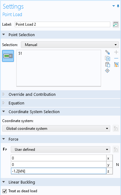
Adding a dead load.
Step 4: Add an Extra Study Step
Insert one more Stationary study step before the Linear Buckling step.
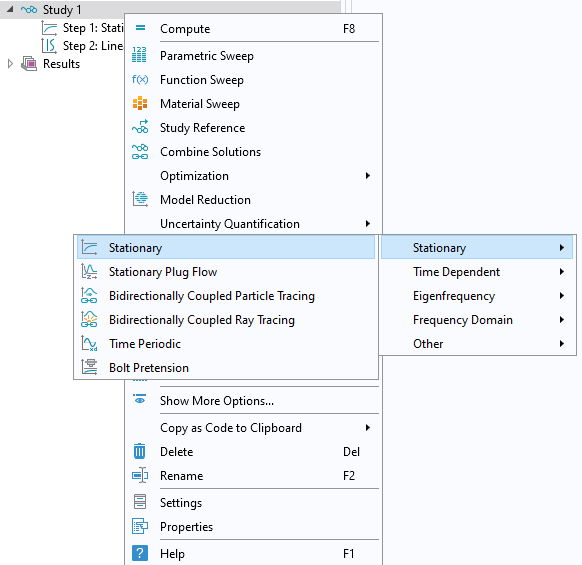
Adding a second Stationary study step.
Step 5: Deactivate Live Loads in One Study Step
In one of the two stationary study steps, you analyze the effect of both loads together. This is just as your model tree is set up.
In the other step, you should analyze only the dead loads. This means that you must disable all load features that describe the live loads, a task most conveniently performed using the Modify model configuration for study step option.
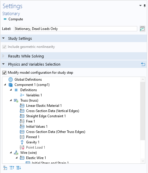
Here, Point Load 1 is disabled.
Step 6: Select the Two Stationary Solutions for the Buckling Analysis
In the Linear Buckling study step settings, you need to specify the two solutions. To do that, you first need to run Show Default Solver for the study. The linearization point is the study with only dead loads, and the live load’s solution contains the sum of live and dead loads.
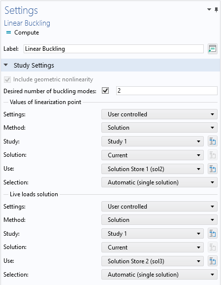
Selecting the two solutions.
Step 7: Run the Whole Study
You may wonder why the static solutions for the two sets of loads are not computed independently. The reason is that if the static solution is nonlinear, the given approach provides a more accurate linearization point for the buckling analysis at the stress state given by the dead load solution.
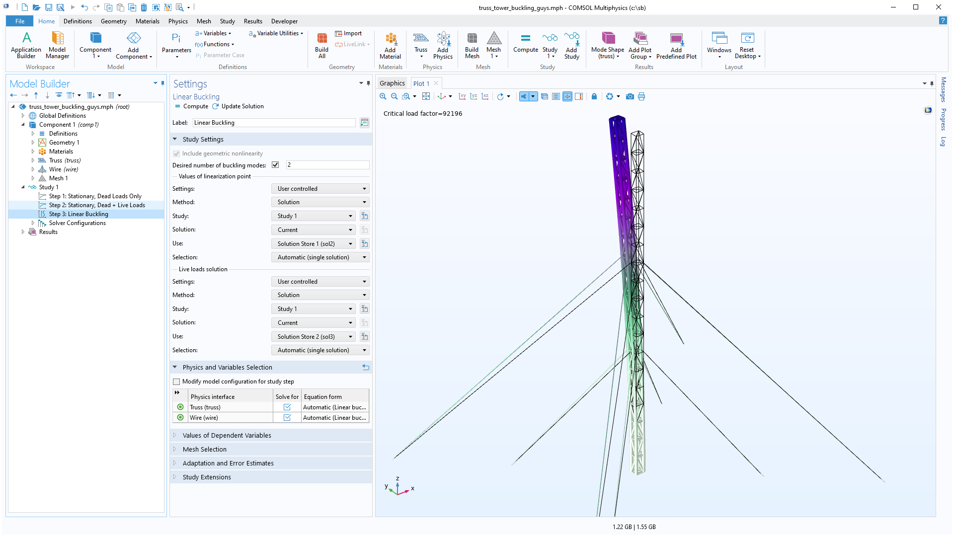
For an example of an analysis of this type, check out the Linear Buckling Analysis of a Truss Tower with Dead Loads model and its related application file. You can find the model and the relevant settings below:
In this example, two effects contribute to the dead load. In addition to the self-weight, there is a pretension in the supporting wires that induces compressive stresses in the lower parts of the tower.
Concluding Remarks
Recent versions of COMSOL Multiphysics make it possible — and easy — to set up advanced buckling studies. Try out the models discussed above by clicking the links below, which will take you to their Application Gallery entries:




Comments (6)
Ivar KJELBERG
January 16, 2023Hi Henrik,
Very nice blog, shell buckling is delicate indeed (and often fatal), full structural too.
I see you are now going far into the details with the buckling, good, just a bit late for me, as I’m been “pushed” to retire, already “overaged”.
But do you have any good reference book(s) / articles to suggest to allow us to test this out on known and discussed cases ?
Sincerely,
Ivar
Henrik Sönnerlind
January 16, 2023 COMSOL EmployeeHi Ivar,
You can find a lot of references and other interesting information about shell buckling on http://shellbuckling.com
Best,
Henrik
Jay Puckett
January 21, 2023Henrik, thanks for writing this blog and demonstrating the new feature. Starting with the simple Euler cantilever is appreciated. In past versions, I typically preloaded to accomplish the estimated preshape. The new feature requires a scale factor for shape(s). This is unnecessarily complex, for the displacement is often known (with a simple computation). Perhaps there could be an option to specify the shape(s)’ max translation [length_units]. So, there would be two methods for input: scaling and absolute units. Jay
Henrik Sönnerlind
January 23, 2023 COMSOL EmployeeThanks for the feedback, Jay.
It would, for sure, be easier to directly provide a displacement
It is, however, not entirely trivial to scale by max displacement for general cases. You would need to specify in which direction it should be measured (this may be in a non-global direction, or maybe the norm should be used). Also, if you want to include more than one mode, you still need to specify the relative size of the contributing modes.
We will look a bit more at this possible option.
Gulzhan Aldan
April 4, 2023Hello,
I am using a linear buckling analysis module to simulate the buckling of thin shells. I wanted to use the first buckling mode as an initial geometric imperfection of the shell and I tried to follow the procedure you outlined in the post. However, I have a question about the load factor you used in buckling imperfection settings. Can it be an arbitrary number and what is its physical meaning?
Thank you very much for your very helpful blogs!
Best,
Gulzhan
Henrik Sönnerlind
April 5, 2023 COMSOL EmployeeHi Gulzhan,
Your comment, to some extent, connects to the one above. The imperfection should have a physical size that is relevant to the problem you are solving. In most cases, that would be controlled by manufacturing imperfections.
The scale factor is a multiplier to the amplitude of the underlying buckling mode (which has an arbitrary scale). So in your case, you need to check the the displacement of the first buckling mode before applying the scale factor.
However, in most cases the effect of changing the scale factor is only that you change the ‘smoothness’ of the postbuckling behavior. A low scale factor will lead to a more pronounced buckling event, sometime to the extent that it is difficult to find convergence.
Regards,
Henrik