Learning Center

Improving Convergence of Nonlinear Stationary Models

---

A nonlinearity can be introduced into a model either in the governing equation or by making any of the material properties, loads, or boundary conditions dependent on the solution. Multiphysics problems are often nonlinear. Stationary (time-invariant) models with nonlinearities may converge very slowly. In this article, we will outline different approaches you can use to improve convergence when solving a nonlinear stationary model.

Approaches for Improving Convergence

The guidance provided here is specific to cases where the iterative solver is used. The algorithm is, generally speaking, a Newton's method approach. That is, when solving, the software starts with the user-specified initial values (found in the Initial Values node) to evaluate all solution-dependent terms. The software then computes an initial solution, and from there it iteratively recomputes the solution, taking into account how these intermediate solutions affect the nonlinearities.

When the difference in the computed solutions between successive iterations is sufficiently small, or when the residual is sufficiently small, the problem is considered to be converged within the specified tolerance. Assuming a well-posed problem, the solver may converge slowly (or not at all) if the initial values are poor, if the nonlinear solver is not able to approach the solution via repeated iterations, or if the mesh is not fine enough to resolve the spatial variations in the solution. The approaches discussed below are options that can be used in such cases.

Specifying Initial Values

The default initial values for the dependent variables in most physics interfaces are zero. The exceptions to this are the heat transfer interfaces, which have a default initial value of 293.15 K, or 20°C, for the temperature fields.

The Initial Values node for the Electric Currents interface (left) and the Heat Transfer in Solids interface (right), displaying the default initial values.

Convergence can be poor when the initial values do not provide a good starting point for the iterative approach described previously. If a good estimate to the solution field is known, this can be entered as an expression in the Initial Value field(s). With the exception of some thermal problems, however, it is often difficult to estimate the solution, so alternative approaches to this are still needed.

Load Ramping

In general, if the loads on a nonlinear system are zero, then the system will be at rest. This means that the solution will also be zero. Thus, an initial value of zero is almost always reasonable if a very small load is applied. Starting from zero-valued initial conditions, the nonlinear solver will most likely converge if a sufficiently small load is applied. We can utilize this in the form of a solving strategy known as load ramping, in which we incrementally increase the loads on a nonlinear system and recompute the model until we have reached the total load. Load ramping is also referred to as a continuation method on the load.

To implement this, you can start by first solving a model with a small but nonzero load. From there, if an additional small load increment is applied, the previously computed solution is a reasonable initial condition. Extending this logic, if you are looking to solve for any arbitrary load on a nonlinear system, such as a multiphysics model, it makes sense to solve a sequence of intermediate problems with gradually increasing load values, and then to use the solutions from each previous step as the initial condition for the next step. This algorithm is known as a continuation method with a Constant predictor (more on this later). The continuation method is enabled by default when using the Auxiliary sweep study extension, as shown below.

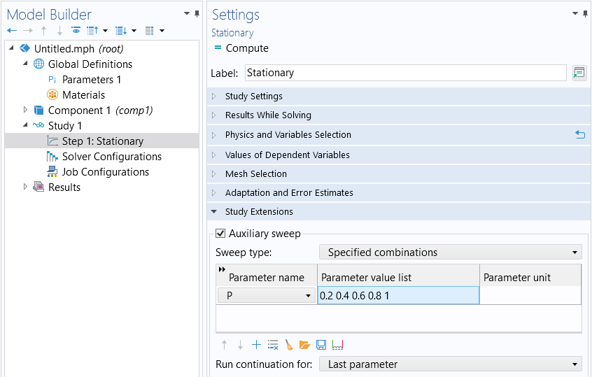
The Auxiliary sweep can be used to implement ramping of any parameter.

A global parameter is introduced (pictured in the figure above, parameter P) to the model by being defined under the Global Definitions node in the Parameters table. It is then ramped from a value of nearly zero up to one. This parameter is used within the physics interfaces to multiply one, some, or all of the applied loads.

The ramping parameter, dT, for a version of the cooling and solidification tutorial model.

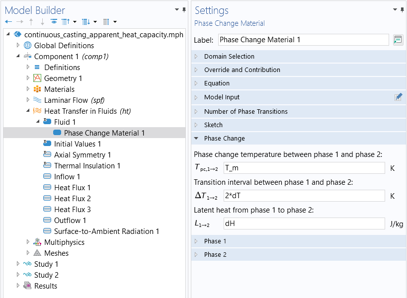
The parameter dT is used within the physics settings under the Heat Transfer in Fluids interface.

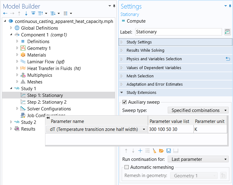
An auxiliary sweep is performed in the first Stationary study step. The ramping parameter dT is used to ramp down from 300 K to 75 K.

The predictor controls how the initial value for the next parameter value is determined. There are three options for predictors: Constant, Linear, and Automatic. The Constant predictor will take the solution from the iteration and use it as the initial value for the iteration. Thus, it uses the solution for the current parameter value as an initial guess, that is,

It is also possible to compute the derivative of the solution with respect to the continuation parameter and use that derivative (evaluated at the iteration) to compute a new initial value of

where is the step size of the continuation parameter. Thus, the initial guess is computed by following the tangent to the solution curve at the current parameter value. This method is known as the continuation method with a Linear predictor and is controlled within the Solver Configurations node in the Parametric node.

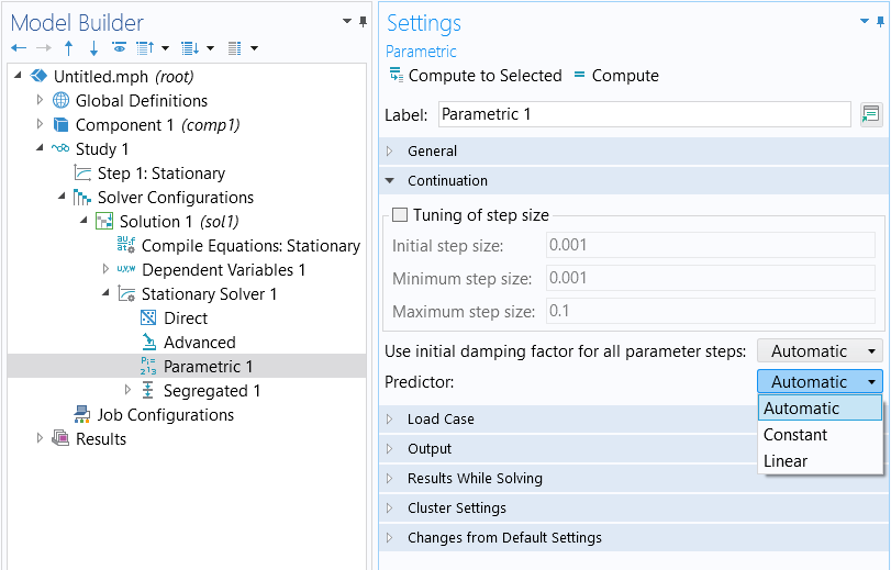
The list of Predictor types to choose from when performing an auxiliary sweep. The default setting is Automatic predictor.

The default Automatic predictor setting will use the Constant predictor when a segregated solution approach is being used. When the fully coupled approach is being used, it will use the Linear predictor. The fully coupled and segregated approaches are discussed further here.

The advantages of the continuation method are twofold. First, it is physically intuitive, often matching how one would perform an experiment. Second, the continuation method will automatically take smaller load increments if a solution cannot be found. For example, if ramping P over values of 0.2, 0.4, 0.6, 0.8, and 1.0, the nonlinear solver may fail to converge for a value of 0.8. In that case, the continuation method will automatically backtrack and solve for intermediate values in the range of 0.6–0.8. This is useful since the software will then return an estimation of the maximum possible load case for which the solver can converge.

Procedure

In summary, the procedure for implementing load ramping for your stationary nonlinear model is:

1. Define a continuation parameter.
2. Multiply one, some, or all of the applied loads by the continuation parameter.
3. Add an auxiliary sweep of the continuation parameter in the Stationary study step.

Nonlinearity Ramping

The technique of load ramping is not always reasonable for all problems. In such cases, you can use the same continuation method but instead ramp the nonlinearities in the model. Nonlinearities arise as a consequence of the governing equation, as a material nonlinear expression, or as a coupling term between physics. To implement this you can once again introduce a global parameter and ramp it from zero to one. You can then use this parameter to modify the nonlinearity expressions in the model. For example, if there is a temperature-dependent material property such as

k(T) = 10[W/m/K]*exp(-(T-293[K])/100[K]),

you can replace it with the expression

k(T,P) = 10[W/m/K]*((1-P)+P*exp(-(T-293[K])/100[K])).

This expression is linear at a value of P=0. At a value of P=1, the expression is equal to the original nonlinear expression. As P is ramped up, the continuation method uses the previous solutions to compute initial conditions for the more nonlinear cases. If you define this nonlinearity ramping so that the first case (P=0) is a purely linear problem, then you are guaranteed to get a solution for this first step of the ramping.

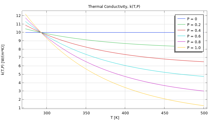
A plot of the temperature-dependent material property, k(T,P), which includes a ramping parameter, P, in the expression. You can observe how the nonlinearity of the material property is ramped up from a value of 0.2 to 1.0. The model file is attached to this article.

Nonlinearity ramping is an especially useful technique if any of the nonlinear terms in your model are very abrupt. One example of an extreme case of nonlinearity could be if you needed to model an instantaneous change in a material property, such as

k(T) = 10[W/m/K]+10[W/m/K]*(T>400[K]).

That is, the material property changes instantaneously from 10W/m/K to 20W/m/K at a temperature value of 400K.

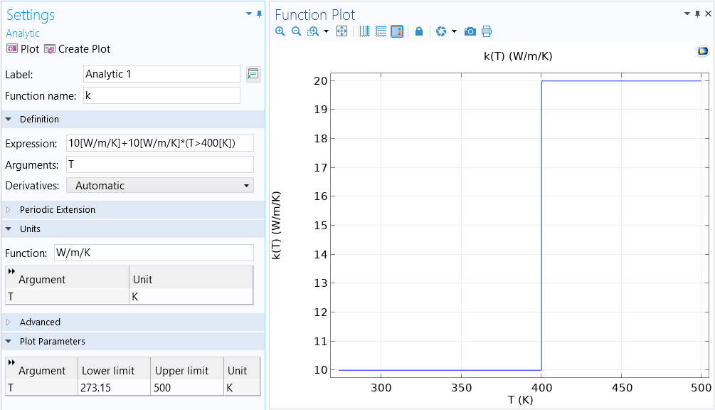
Plot of the temperature-dependent material property, k(T). The instantaneous change at 400 K results in the property being highly nonlinear.

This case is generally difficult or impossible to solve since the material property is not smooth. Instead, you can use a nonlinear material property expression that ramps from a very smooth function to one that is nearly discontinuous. The continuation method will backtrack again and solve for the intermediate values of the ramping parameter, giving you the closest approximation to the abrupt transition.

We can create a smooth step transition at the nonlinearity at 400 K using the Step function:

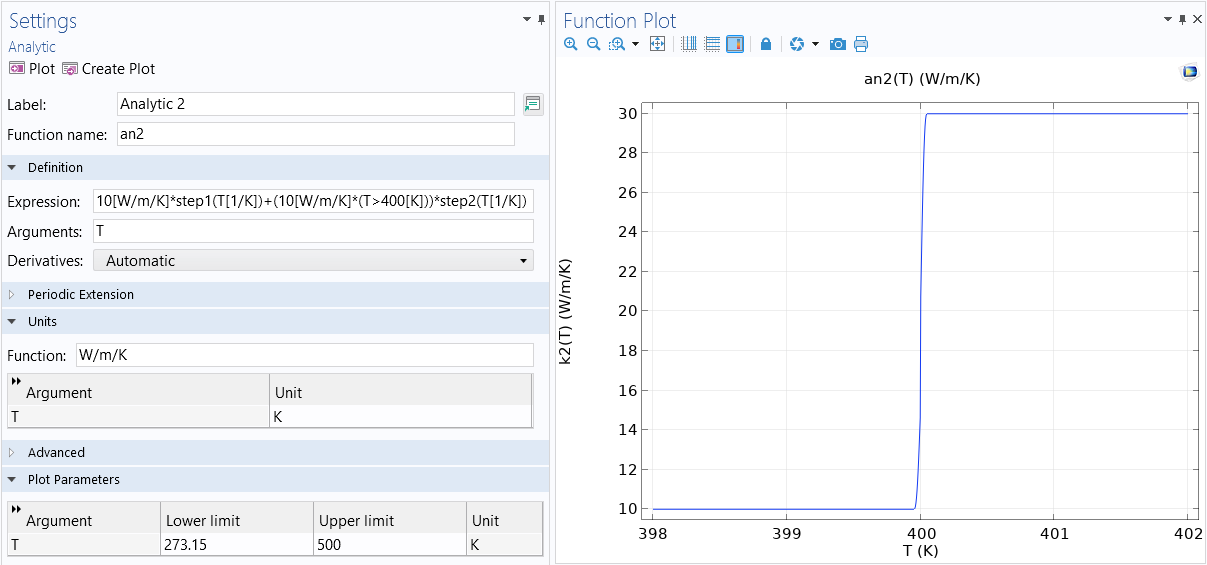The nonlinearity in the material property is smoothed out using multiple Step functions.

We can also use a function that includes smoothing, such as a Piecewise function:

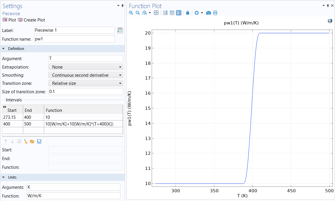The nonlinearity in the material property k(T) is smoothed out using a Piecewise function. Both this function and the Step function used to implement smoothing are available in the model file, which is attached to this article.

Load ramping and nonlinearity ramping can be used in combination, but start with only one or a few of the loads or nonlinearities being ramped. Check the solver log to see if the continuation method is backtracking. If so, use a finer increment in that range.

Procedure

In summary, the procedure for implementing nonlinearity ramping in your stationary nonlinear model is:

1. Define a ramping parameter or smoothing function.
2. Multiply the nonlinearity by the ramping parameter or smoothing function.
3. Add an auxiliary sweep of the ramping parameter in the Stationary study step.

Alternatively, you can use a function to implement smoothing at or for the nonlinearity by taking the following steps:

1. Define a smoothing function.
2. Multiply the nonlinearity by the smoothing function.

Mesh Refinement

If both load ramping and nonlinearity ramping are still leading to slow convergence, another approach for improving the convergence is to refine the mesh. The finite element mesh must be fine enough to resolve the spatial variations in the solution fields. Ideally, one would use small elements in regions where the solution varies quickly in space, and larger elements elsewhere. However, it is usually not possible to know where these regions are ahead of time. Therefore, it is recommended to use adaptive mesh refinement, which will automatically refine the mesh only in the regions where it is needed and coarsen the mesh elsewhere. It is also possible to manually refine the mesh. For more details, see Performing a Mesh Refinement Study.

Mesh refinement may often need to be combined with load or nonlinearity ramping and may require a set of studies. First, start with a relatively coarse mesh for nonlinearity ramping, then refine the mesh and ramp further on the refined mesh. An example model that combines the techniques of nonlinearity ramping and adaptive mesh refinement with multiple study steps is the Cooling and Solidification of Metal tutorial model, which was highlighted earlier in this article.

Solution Approach

There are two types of approaches that can be used when iteratively solving the nonlinear system of equations, a fully coupled or segregated approach. The fully coupled approach solves for all unknowns in the problem at once, whereas the segregated approach solves sets of unknowns separately. Consequently, the fully coupled approach provides the most robust convergence generally, while the segregated approach can converge robustly as long as there are not strong couplings between the physics in your multiphysics model. If you are encountering convergence issues it may be optimal to switch the approach being used to solve the model equations. Note, however, that there are occasional exceptions to this rule. For example, k-epsilon turbulent flow is more robust with the segregated approach.

To switch between these solver types, go to the Stationary Solver node under the Study node. There will always already be either a Segregated or Fully Coupled feature beneath this. Right-click on the Stationary Solver node and add either the Segregated or Fully Coupled feature.

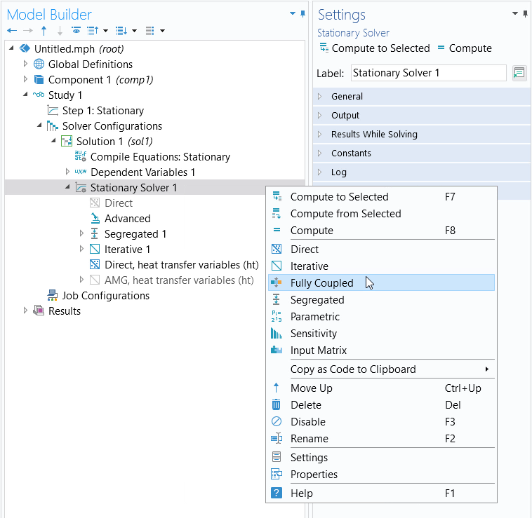
The Stationary Solver node, where you can switch between using the Fully Coupled and Segregated approach.

Within either of these features it can also be helpful to enable the Results While Solving option (shown below) to visualize the iterations being taken during the solution.

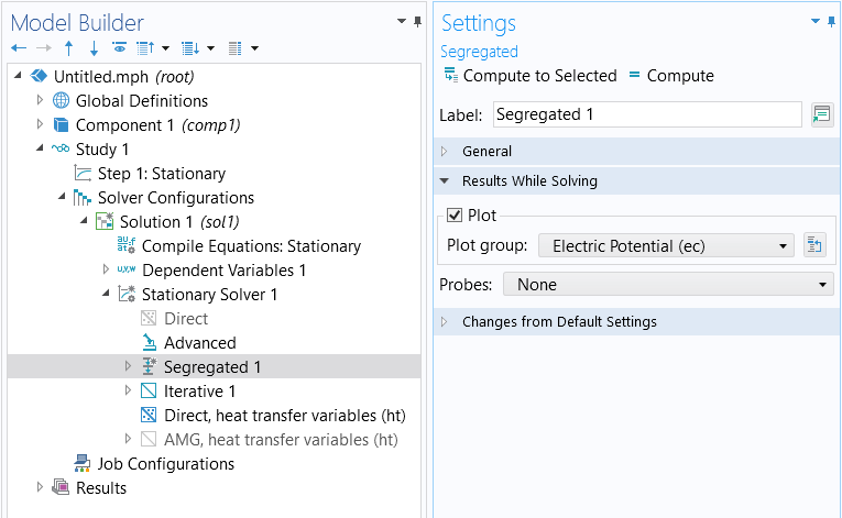
The settings for the Results While Solving section.

General Approach for Model Checking

If it is not clear that any of the abovementioned strategies are working, it is useful to take a more general approach to verify the general validity of your model. This involves a systematic reduction in the model complexity. The objective is to simplify the model to a state where the model will solve but with linear approximations. From there, you gradually reintroduce the nonlinearities of the model as you recompute it to identify what is contributing to any convergence issues with your model when solving.

Examine the model and identify all terms that introduce nonlinearities, such as multiphysics couplings, nonlinear materials relationships, and nonlinear boundary conditions. With respect to any nonlinearities, replace them by a reasonable linearized term. Repeat this for every nonlinearity of the model. With respect to multiphysics couplings, rather than solving the problem using a fully coupled approach (the default), solve the problem sequentially, with one physics being solved after another. You can also use the manual approach with predefined couplings to simplify and break up your multiphysics model into multiple standalone analyses. The objective here is to simplify the model to a state where the model will solve with linear approximations. With sufficient simplification, a model can be reduced to a linear problem, and if this simplified model does not converge, you can refer to our resource on what to do when a linear stationary model is not solving.

Once a simplified solvable version of the model has been found, gradually increase the model complexity again, reintroducing nonlinearities and multiphysics couplings. Using this technique systematically, along with the techniques described previously, typically makes it possible to identify the nonlinearities in the model that are leading to issues. It may also reveal that the model itself is ill-posed in some way. Sometimes, reducing the model complexity can be quite challenging, and it can be better to start from as simple of a case as possible and then gradually increase the complexity.

Converting to a Time-Dependent Formulation

If you have tried the approaches mentioned here and are certain that the problem itself is well posed, you should consider that the nonlinear problem may not, in fact, have a stationary (time-invariant) solution. A classic example of this is fluid flow around a cylinder with high but constant flow rates. At low flow speeds, the flow solution will be time invariant, but at higher flow rates there will be vortex shedding, a time-varying change in the flow field behind the cylinder. Such problems can be solved in the time domain using a Time Dependent study.

The Flow Past a Cylinder tutorial model, wherein the flow rate around the cylinder results in vortex shedding.

The difference in flow velocity for the Flow Past a Cylinder tutorial model where a significantly lower inlet velocity is specified.

In such cases, it will be particularly helpful to ramp up the load gradually from consistent initial values. Ramping the nonlinearities over time is not as strongly motivated, but step changes in nonlinearities should be smoothed out throughout the simulation. You can use either a very fine mesh throughout the simulation domain or use adaptive mesh refinement.

Further Learning

• Load ramping:
  • Blog post: Load Ramping of Nonlinear Problems
• Nonlinearity ramping:
  • Blog post: How to Solve a Classic CFD Benchmark: The Lid-Driven Cavity Problem
  • Blog post: Nonlinearity Ramping for Improving Convergence of Nonlinear Problems
  • Blog post: Viscosity Ramping Improves the Convergence of CFD Models
  • Documentation: Specifying Discontinuous Functions section in the COMSOL Multiphysics Reference Manual